Template:Weibull parameters maximum likelihood estimation: Difference between revisions
| Line 8: | Line 8: | ||
'''Solution''' | |||
In this case, we have non-grouped data with no suspensions or intervals, i.e. complete data. The equations for the partial derivatives of the log-likelihood function are derived in Appendix C and given next: | In this case, we have non-grouped data with no suspensions or intervals, i.e. complete data. The equations for the partial derivatives of the log-likelihood function are derived in Appendix C and given next: | ||
::<math> \frac{\partial \Lambda }{\partial \beta }=\frac{6}{\beta } +\sum_{i=1}^{6}\ln \left( \frac{T_{i}}{\eta }\right) -\sum_{i=1}^{6}\left( \frac{T_{i}}{\eta }\right) ^{\beta }\ln \left( \frac{T_{i}}{\eta }\right) =0 | ::<math> \frac{\partial \Lambda }{\partial \beta }=\frac{6}{\beta } +\sum_{i=1}^{6}\ln \left( \frac{T_{i}}{\eta }\right) -\sum_{i=1}^{6}\left( \frac{T_{i}}{\eta }\right) ^{\beta }\ln \left( \frac{T_{i}}{\eta }\right) =0 | ||
Revision as of 17:45, 9 February 2012
Maximum Likelihood Estimation
As outlined in Chapter 3, maximum likelihood estimation works by developing a likelihood function based on the available data and finding the values of the parameter estimates that maximize the likelihood function. This can be achieved by using iterative methods to determine the parameter estimate values that maximize the likelihood function, but this can be rather difficult and time-consuming, particularly when dealing with the three-parameter distribution. Another method of finding the parameter estimates involves taking the partial derivatives of the likelihood function with respect to the parameters, setting the resulting equations equal to zero and solving simultaneously to determine the values of the parameter estimates. ( Note that MLE asymptotic properties do not hold when estimating γ using MLE [27].) The log-likelihood functions and associated partial derivatives used to determine maximum likelihood estimates for the Weibull distribution are covered in Appendix C.
Maximum Likelihood Estimation Example
Repeat Example 1 using maximum likelihood estimation.
Solution
In this case, we have non-grouped data with no suspensions or intervals, i.e. complete data. The equations for the partial derivatives of the log-likelihood function are derived in Appendix C and given next:
- [math]\displaystyle{ \frac{\partial \Lambda }{\partial \beta }=\frac{6}{\beta } +\sum_{i=1}^{6}\ln \left( \frac{T_{i}}{\eta }\right) -\sum_{i=1}^{6}\left( \frac{T_{i}}{\eta }\right) ^{\beta }\ln \left( \frac{T_{i}}{\eta }\right) =0 }[/math]
- and:
- [math]\displaystyle{ \frac{\partial \Lambda }{\partial \eta }=\frac{-\beta }{\eta }\cdot 6+\frac{ \beta }{\eta }\sum\limits_{i=1}^{6}\left( \frac{T_{i}}{\eta }\right) ^{\beta }=0 }[/math]
Solving the above equations simultaneously we get:
- [math]\displaystyle{ \hat{\beta }=1.933, }[/math] [math]\displaystyle{ \hat{\eta }=73.526 }[/math]
The variance/covariance matrix is found to be,
- [math]\displaystyle{ \left[ \begin{array}{ccc} \hat{Var}\left( \hat{\beta }\right) =0.4211 & \hat{Cov}( \hat{\beta },\hat{\eta })=3.272 \\ \hat{Cov}(\hat{\beta },\hat{\eta })=3.272 & \hat{Var} \left( \hat{\eta }\right) =266.646 \end{array} \right] }[/math]
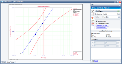
The results and the associated graph using Weibull++ (MLE) are shown next.
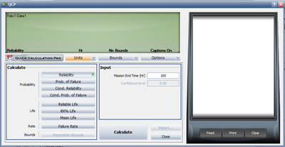
You can view the variance/covariance matrix directly by clicking the Quick Calculation Pad (QCP) icon
Note that the decimal accuracy displayed and used is based on your individual User Setup.

