Template:Example: Weibull MLE: Difference between revisions
Jump to navigation
Jump to search
No edit summary |
No edit summary |
||
| Line 2: | Line 2: | ||
Repeat [[Weibull Example 1 Data|Example 1]] using maximum likelihood estimation. | Repeat [[Weibull Example 1 Data|Example 1]] using maximum likelihood estimation. | ||
'''Solution''' | '''Solution''' | ||
| Line 18: | Line 17: | ||
::<math> \hat{\beta }=1.933,</math> <math>\hat{\eta }=73.526 </math> | ::<math> \hat{\beta }=1.933,</math> <math>\hat{\eta }=73.526 </math> | ||
The variance/covariance matrix is found to be, | The variance/covariance matrix is found to be, | ||
| Line 33: | Line 31: | ||
[[Image: Weibull Distribution Example 5 Variance Matrix.png|center|450px| ]] | [[Image: Weibull Distribution Example 5 Variance Matrix.png|center|450px| ]] | ||
Note that the decimal accuracy displayed and used is based on your individual Application Setup. | |||
Revision as of 02:12, 8 August 2012
Maximum Likelihood Estimation Example
Repeat Example 1 using maximum likelihood estimation.
Solution
In this case, we have non-grouped data with no suspensions or intervals, (i.e., complete data). The equations for the partial derivatives of the log-likelihood function are derived in an appendix and given next:
- [math]\displaystyle{ \frac{\partial \Lambda }{\partial \beta }=\frac{6}{\beta } +\sum_{i=1}^{6}\ln \left( \frac{T_{i}}{\eta }\right) -\sum_{i=1}^{6}\left( \frac{T_{i}}{\eta }\right) ^{\beta }\ln \left( \frac{T_{i}}{\eta }\right) =0 }[/math]
- and:
- [math]\displaystyle{ \frac{\partial \Lambda }{\partial \eta }=\frac{-\beta }{\eta }\cdot 6+\frac{ \beta }{\eta }\sum\limits_{i=1}^{6}\left( \frac{T_{i}}{\eta }\right) ^{\beta }=0 }[/math]
Solving the above equations simultaneously we get:
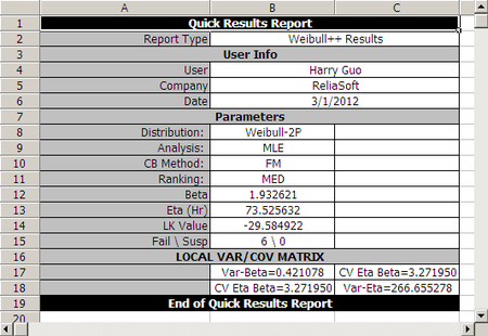
- [math]\displaystyle{ \hat{\beta }=1.933, }[/math] [math]\displaystyle{ \hat{\eta }=73.526 }[/math]
The variance/covariance matrix is found to be,
- [math]\displaystyle{ \left[ \begin{array}{ccc} \hat{Var}\left( \hat{\beta }\right) =0.4211 & \hat{Cov}( \hat{\beta },\hat{\eta })=3.272 \\ \hat{Cov}(\hat{\beta },\hat{\eta })=3.272 & \hat{Var} \left( \hat{\eta }\right) =266.646 \end{array} \right] }[/math]
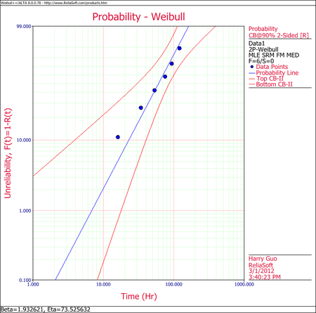
The results and the associated graph using Weibull++ (MLE) are shown next.

You can view the variance/covariance matrix directly by clicking the Analysis Summary at the Main Panel.

Note that the decimal accuracy displayed and used is based on your individual Application Setup.