This example compares the results of a cumulative damage model for a step stress test.
Reference Case
The data set is from Table 2.1 on page 496 in the book Accelerated Testing: Statistical Models, Test Plans, and Data Analysis by Dr. Nelson, John Wiley & Sons, 1990.
Data
A step-stress test is conducted for one type of cable insulation to estimate the insulation life at a constant design stress of 400 volts/mil. The test cables are of different thickness in unit of mils (0.001 inch). The stress is the applied step voltage divided by the thickness. A total of 6 step-stress profiles are used. These stress profiles are calculated based the applied voltage (Kilovolts) and the insulation thickness given on page 495 and Table 2.1. For all the profiles, the holding time is 10 mins for the first 4 steps. From step 5, different a holding time is applied at each step for each of the stress profiles. These profiles are given in the following tables.
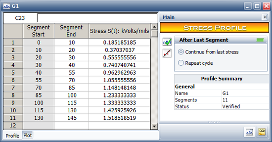
Profile 1 (named "G1"): Holding time is 15 mins after step 4 and the thickness is 27 mils.
| Segment Start Time
|
Segment End Time
|
Stress (Kvolts/mils)
|
| 0 |
10 |
0.185185185
|
| 10 |
20 |
0.37037037
|
| 20 |
30 |
0.555555556
|
| 30 |
40 |
0.740740741
|
| 40 |
55 |
0.962962963
|
| 55 |
70 |
1.055555556
|
| 70 |
85 |
1.148148148
|
| 85 |
100 |
1.233333333
|
| 100 |
115 |
1.333333333
|
| 115 |
130 |
1.425925926
|
| 130 |
145 |
1.518518519
|
Profile 2 (named "G2"): Holding time is 60 mins after step 4 and the thickness is 29.5 mils.
| Segment Start Time
|
Segment End Time
|
Stress (Kvolts/mils)
|
| 0 |
10 |
0.169491525
|
| 10 |
20 |
0.338983051
|
| 20 |
30 |
0.508474576
|
| 30 |
40 |
0.677966102
|
| 40 |
100 |
0.881355932
|
| 100 |
160 |
0.966101695
|
| 160 |
220 |
1.050847458
|
| 220 |
280 |
1.128813559
|
| 280 |
340 |
1.220338983
|
| 340 |
400 |
1.305084746
|
| 400 |
460 |
1.389830508
|
Profile 3 (named "G3"): Holding time is 60 mins after step 4 and the thickness is 28 mils.
| Segment Start Time
|
Segment End Time
|
Stress (Kvolts/mils)
|
| 0 |
10 |
0.178571429
|
| 10 |
20 |
0.357142857
|
| 20 |
30 |
0.535714286
|
| 30 |
40 |
0.714285714
|
| 40 |
100 |
0.928571429
|
| 100 |
160 |
1.017857143
|
| 160 |
220 |
1.107142857
|
| 220 |
280 |
1.189285714
|
| 280 |
340 |
1.285714286
|
| 340 |
400 |
1.375
|
| 400 |
460 |
1.464285714
|
Profile 4 (named "G4"): Holding time is 240 mins after step 4 and the thickness is 29 mils.
| Segment Start Time
|
Segment End Time
|
Stress (Kvolts/mils)
|
| 0 |
10 |
0.172413793
|
| 10 |
20 |
0.344827586
|
| 20 |
30 |
0.517241379
|
| 30 |
40 |
0.689655172
|
| 40 |
280 |
0.896551724
|
| 280 |
520 |
0.982758621
|
| 520 |
760 |
1.068965517
|
| 760 |
1000 |
1.148275862
|
| 1000 |
1240 |
1.24137931
|
| 1240 |
1480 |
1.327586207
|
| 1480 |
1720 |
1.413793103
|
Profile 5 (named "G5"): Holding time is 240 mins after step 4 and the thickness is 30 mils.
| Segment Start Time
|
Segment End Time
|
Stress (Kvolts/mils)
|
| 0 |
10 |
0.166666667
|
| 10 |
20 |
0.333333333
|
| 20 |
30 |
0.5
|
| 30 |
40 |
0.666666667
|
| 40 |
280 |
0.866666667
|
| 280 |
520 |
0.95
|
| 520 |
760 |
1.033333333
|
| 760 |
1000 |
1.11
|
| 1000 |
1240 |
1.2
|
| 1240 |
1480 |
1.283333333
|
| 1480 |
1720 |
1.366666667
|
Profile 6 (named "G6"): Holding time is 960 mins after step 4 and the thickness is 30 mils.
| Segment Start Time
|
Segment End Time
|
Stress (Kvolts/mils)
|
| 0 |
10 |
0.166666667
|
| 10 |
20 |
0.333333333
|
| 20 |
30 |
0.5
|
| 30 |
40 |
0.666666667
|
| 40 |
1000 |
0.866666667
|
| 1000 |
1960 |
0.95
|
| 1960 |
2920 |
1.033333333
|
| 2920 |
3880 |
1.11
|
| 3880 |
4840 |
1.2
|
| 4840 |
5800 |
1.283333333
|
| 5800 |
6760 |
1.366666667
|
The following table shows the test results.
| Status F/S
|
Time to F/S
|
Test Profile
|
Subset ID
|
| F |
102 |
G1 |
1
|
| F |
113 |
G1 |
2
|
| F |
113 |
G1 |
3
|
| S |
370 |
G2 |
4
|
| F |
345 |
G2 |
5
|
| S |
345 |
G3 |
6
|
| F |
1249 |
G4 |
7
|
| F |
1333 |
G4 |
8
|
| S |
1333 |
G4 |
9
|
| F |
1096.6 |
G4 |
10
|
| F |
1250.8 |
G5 |
11
|
| F |
1097.9 |
G4 |
12
|
| F |
2460.9 |
G6 |
13
|
| S |
2460.9 |
G6 |
14
|
| F |
2700.4 |
G6 |
15
|
| F |
2923.9 |
G6 |
16
|
| F |
1160 |
G6 |
17
|
| F |
1962.9 |
G6 |
18
|
| S |
363.9 |
G6 |
19
|
| F |
898.4 |
G6 |
20
|
| F |
4142.1 |
G6 |
21
|
Result
The power law life stress relationship and the Weibull distribution is used for the data. At a constant stress V, the [math]\displaystyle{ \eta\,\! }[/math] is:
- [math]\displaystyle{ \eta(V) = \left(\frac{V_{0}}{V} \right)^p\,\! }[/math]
where [math]\displaystyle{ V_{0}\,\! }[/math] and [math]\displaystyle{ p\,\! }[/math] are the model parameters used in the book.
The above equation can be rewritten as:
- [math]\displaystyle{ \eta(V) = e^{\alpha_{0}+\alpha_{1}ln(V)}\,\! }[/math]
where [math]\displaystyle{ \alpha_{0} = pln(V_{0})\,\! }[/math] and [math]\displaystyle{ \alpha_{1} = -p\,\! }[/math]
The reliability function at time t is stress V is:
- [math]\displaystyle{ R(t,V) = e^{-\left(\frac{t}{\eta(V)} \right)^\beta}\,\! }[/math]
When stress is varying with time, the reliability at time t is given as:
- [math]\displaystyle{ R(t,V) = e^{-\left(\int_{0}^{t}\frac{1}{\eta(x)} dx\right)^{\beta}}\,\! }[/math]
In the book, the following results are provided:
- ML solution for the parameters are [math]\displaystyle{ \beta\,\! }[/math] = 0.75597, [math]\displaystyle{ V_{0}\,\! }[/math] = 1616.4 (1.6164 Kvolts), and [math]\displaystyle{ p\,\! }[/math] = 19.937.
- The maximum log likelihood is -103.53.
- The 1% percentile point (B1 life) at 0.4 Kvolts/mil is 2.81 x 10⁹.
- The normal distribution approximation two-sided 95% confidence intervals are [math]\displaystyle{ \beta\,\! }[/math] = [0.18, 1.33], [math]\displaystyle{ V_{0}\,\! }[/math] = [1291, 1941.8], [math]\displaystyle{ p\,\! }[/math] = [6.2, 33.7], and the B1 life is [2.65 x 10⁴, 2.98 x 10¹⁴].
Results in ALTA
First, we create each stress profile in ALTA. For example, the following picture shows the data for Profile G1.
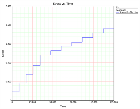
The following picture shows the plot for this stress profile.
The next step is to enter the failure data into an ALTA standard folio and then use the stress profiles to define the stress values, as shown next.

