Cumulative Damage Model for Step Stress Profiles: Difference between revisions

From ReliaWiki
Jump to navigation Jump to search
No edit summary
No edit summary
Line 303: Line 303:


The next step is to enter the failure data into an ALTA standard folio and then use the stress profiles to define the stress values, as shown next.
The next step is to enter the failure data into an ALTA standard folio and use the stress profiles to define the stress values, as shown next.
 
[[Image: Step Stress_folio.png|center]]
 
 
The log transformation is used for the stress. To compare the parameter values used in the book with the results obtained by ALTA, we need do convert the values in the book in terms of the parameters used in ALTA. Therefore the parameters in the book are: <math>\beta\,\!</math> = 0.75597, &nbsp; <math>\alpha_{0}\,\!</math> = 9.573776, &nbsp; <math>\alpha_{1}\,\!</math> = -19.937. Comparing these values to the value shown in the picture above, we see that the results obtained in ALTA are close to the results shown in the book.
 
The picture above also shows that the maximum log likelihood (LK Value) is -114.932651. This value is smaller than the value given in the book. To validate what the LK value would be if the results in the book were used in ALTA, we use the Alter Parameters tool, as shown next.
 
[[Image: Step Stress_alter parameters.png|center]] 
 
 
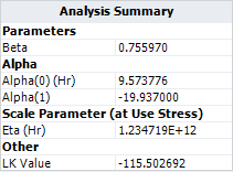
The resulting LK Value is -115.502692, as shown next.
 
[[Image: Step Stress_alter parameters results.png|center|Altered Parameters]]
<center>Altered Parameters</center>
 
 
This value is different from the value of -13.53 given in the book. Later, we will validate the calculations for this result.
 
Using the parameters values originally calculated in ALTA:
 
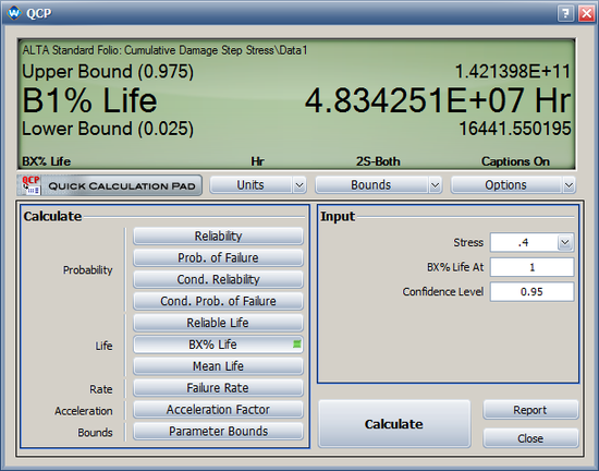
* The 1% percentile point (B1 life) at 0.4 Kvolts/mil is 4.8342 X 10<sup>7</sup> hours, as shown next.
 
[[Image: Step Stress qcp.png|center|550px]]
 
 
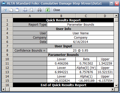
* The 2-sided 95% confidence intervals for model parameters are shown next.
 
[[Image: Step Stress bounds.png|center]]
 
 
'''Validate the Likelihood Calculation in ALTA'''

Revision as of 18:07, 16 June 2014

ALTA Reference Examples Banner.png


New format available! This reference is now available in a new format that offers faster page load, improved display for calculations and images and more targeted search.

As of January 2024, this Reliawiki page will not continue to be updated. Please update all links and bookmarks to the latest references at ALTA examples and ALTA reference examples.

Cumulative Damage Model for Step Stress Profiles

This example compares the results of a cumulative damage model for a step stress test.


Reference Case

The data set is from Table 2.1 on page 496 in the book Accelerated Testing: Statistical Models, Test Plans, and Data Analysis by Dr. Nelson, John Wiley & Sons, 1990.


Data

A step-stress test is conducted for one type of cable insulation to estimate the insulation life at a constant design stress of 400 volts/mil. The test cables are of different thickness, in unit of mils (0.001 inch). The stress is the applied step voltage divided by the thickness.

A total of 6 step-stress profiles are used. These stress profiles are calculated based on the applied voltage (Kilovolts) and the insulation thickness given on page 495 and Table 2.1. For all the stress profiles, the holding time for the first 4 steps is 10 mins. From step 5 onwards, a different a holding time is applied at each step for each of the stress profiles. These profiles are given in the following tables.


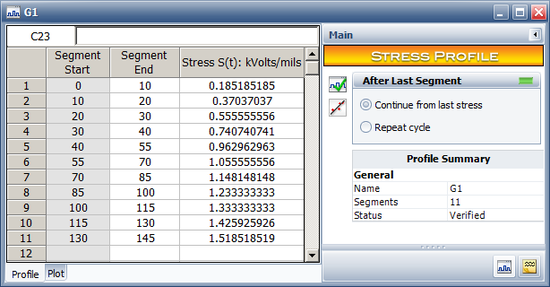
Profile 1 (named "G1"): The holding time after step 4 is 15 mins and the thickness is 27 mils.

Segment Start Time Segment End Time Stress (Kvolts/mils)
0 10 0.185185185
10 20 0.37037037
20 30 0.555555556
30 40 0.740740741
40 55 0.962962963
55 70 1.055555556
70 85 1.148148148
85 100 1.233333333
100 115 1.333333333
115 130 1.425925926
130 145 1.518518519


Profile 2 (named "G2"): The holding time after step 4 is 60 mins and the thickness is 29.5 mils.

Segment Start Time Segment End Time Stress (Kvolts/mils)
0 10 0.169491525
10 20 0.338983051
20 30 0.508474576
30 40 0.677966102
40 100 0.881355932
100 160 0.966101695
160 220 1.050847458
220 280 1.128813559
280 340 1.220338983
340 400 1.305084746
400 460 1.389830508

Profile 3 (named "G3"): The holding time after step 4 is 60 mins and the thickness is 28 mils.

Segment Start Time Segment End Time Stress (Kvolts/mils)
0 10 0.178571429
10 20 0.357142857
20 30 0.535714286
30 40 0.714285714
40 100 0.928571429
100 160 1.017857143
160 220 1.107142857
220 280 1.189285714
280 340 1.285714286
340 400 1.375
400 460 1.464285714

Profile 4 (named "G4"): The holding time after step 4 is 240 mins and the thickness is 29 mils.

Segment Start Time Segment End Time Stress (Kvolts/mils)
0 10 0.172413793
10 20 0.344827586
20 30 0.517241379
30 40 0.689655172
40 280 0.896551724
280 520 0.982758621
520 760 1.068965517
760 1000 1.148275862
1000 1240 1.24137931
1240 1480 1.327586207
1480 1720 1.413793103

Profile 5 (named "G5"): The holding time after step 4 is 240 mins and the thickness is 30 mils.

Segment Start Time Segment End Time Stress (Kvolts/mils)
0 10 0.166666667
10 20 0.333333333
20 30 0.5
30 40 0.666666667
40 280 0.866666667
280 520 0.95
520 760 1.033333333
760 1000 1.11
1000 1240 1.2
1240 1480 1.283333333
1480 1720 1.366666667

Profile 6 (named "G6"): The holding time after step 4 is 960 mins and the thickness is 30 mils.

Segment Start Time Segment End Time Stress (Kvolts/mils)
0 10 0.166666667
10 20 0.333333333
20 30 0.5
30 40 0.666666667
40 1000 0.866666667
1000 1960 0.95
1960 2920 1.033333333
2920 3880 1.11
3880 4840 1.2
4840 5800 1.283333333
5800 6760 1.366666667

The following table shows the test results.

Status F/S Time to F/S Test Profile Subset ID
F 102 G1 1
F 113 G1 2
F 113 G1 3
S 370 G2 4
F 345 G2 5
S 345 G3 6
F 1249 G4 7
F 1333 G4 8
S 1333 G4 9
F 1096.6 G4 10
F 1250.8 G5 11
F 1097.9 G4 12
F 2460.9 G6 13
S 2460.9 G6 14
F 2700.4 G6 15
F 2923.9 G6 16
F 1160 G6 17
F 1962.9 G6 18
S 363.9 G6 19
F 898.4 G6 20
F 4142.1 G6 21

Result

The power law life stress relationship and the Weibull distribution is used to analyze the data. At a constant stress V, the [math]\displaystyle{ \eta\,\! }[/math] is:

[math]\displaystyle{ \eta(V) = \left(\frac{V_{0}}{V} \right)^p\,\! }[/math]


where [math]\displaystyle{ V_{0}\,\! }[/math] and [math]\displaystyle{ p\,\! }[/math] are the model parameters used in the book.


The above equation can be rewritten as:

[math]\displaystyle{ \eta(V) = e^{\alpha_{0}+\alpha_{1}ln(V)}\,\! }[/math]


where [math]\displaystyle{ \alpha_{0} = pln(V_{0})\,\! }[/math]  and  [math]\displaystyle{ \alpha_{1} = -p\,\! }[/math]


The reliability function at time t and stress V is:

[math]\displaystyle{ R(t,V) = e^{-\left(\frac{t}{\eta(V)} \right)^\beta}\,\! }[/math]


When stress is varying with time, the reliability at time t is given as:

[math]\displaystyle{ R(t,V) = e^{-\left(\int_{0}^{t}\frac{1}{\eta(x)} dx\right)^{\beta}}\,\! }[/math]


In the book, the following results are provided:

  • ML solution for the parameters are [math]\displaystyle{ \beta\,\! }[/math] = 0.75597, [math]\displaystyle{ V_{0}\,\! }[/math] = 1616.4 (1.6164 Kvolts), and [math]\displaystyle{ p\,\! }[/math] = 19.937.
  • The maximum log likelihood is -103.53.
  • The 1% percentile point (B1 life) at 0.4 Kvolts/mil is 2.81 x 10⁹.
  • The normal distribution approximation two-sided 95% confidence intervals are [math]\displaystyle{ \beta\,\! }[/math] = [0.18, 1.33], [math]\displaystyle{ V_{0}\,\! }[/math] = [1291, 1941.8], [math]\displaystyle{ p\,\! }[/math] = [6.2, 33.7], and the B1 life is [2.65 x 10⁴, 2.98 x 10¹⁴].


Results in ALTA

First, we create each stress profile in ALTA. For example, the following picture shows the data for Profile G1.

Step Stress G1.png


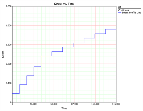
The following picture shows the plot for this stress profile.

Step Stress G1 plot.png


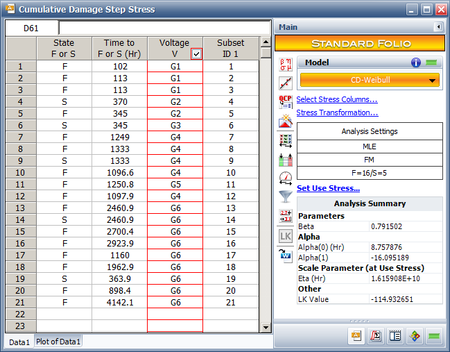
The next step is to enter the failure data into an ALTA standard folio and use the stress profiles to define the stress values, as shown next.

Step Stress folio.png


The log transformation is used for the stress. To compare the parameter values used in the book with the results obtained by ALTA, we need do convert the values in the book in terms of the parameters used in ALTA. Therefore the parameters in the book are: [math]\displaystyle{ \beta\,\! }[/math] = 0.75597,   [math]\displaystyle{ \alpha_{0}\,\! }[/math] = 9.573776,   [math]\displaystyle{ \alpha_{1}\,\! }[/math] = -19.937. Comparing these values to the value shown in the picture above, we see that the results obtained in ALTA are close to the results shown in the book.

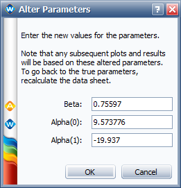
The picture above also shows that the maximum log likelihood (LK Value) is -114.932651. This value is smaller than the value given in the book. To validate what the LK value would be if the results in the book were used in ALTA, we use the Alter Parameters tool, as shown next.

Step Stress alter parameters.png


The resulting LK Value is -115.502692, as shown next.

Altered Parameters
Altered Parameters


This value is different from the value of -13.53 given in the book. Later, we will validate the calculations for this result.

Using the parameters values originally calculated in ALTA:

  • The 1% percentile point (B1 life) at 0.4 Kvolts/mil is 4.8342 X 10⁷ hours, as shown next.
Step Stress qcp.png


  • The 2-sided 95% confidence intervals for model parameters are shown next.
Step Stress bounds.png


Validate the Likelihood Calculation in ALTA