Probability Plotting: Difference between revisions
Steve Sharp (talk | contribs) No edit summary |
Steve Sharp (talk | contribs) No edit summary |
||
| Line 12: | Line 12: | ||
data, using probability plotting, are as follows: | data, using probability plotting, are as follows: | ||
<br> | <br> | ||
:• Rank the times-to-failure in ascending order as shown next. | ::• Rank the times-to-failure in ascending order as shown next. | ||
<br> | <br> | ||
| Line 27: | Line 27: | ||
<br> | <br> | ||
:• Obtain their median rank plotting positions. | ::• Obtain their median rank plotting positions. | ||
<br> | <br> | ||
Median rank positions are used instead of other ranking methods because median ranks are at a | Median rank positions are used instead of other ranking methods because median ranks are at a | ||
specific confidence level (50%). | specific confidence level (50%). | ||
<br> | <br> | ||
:• The times-to-failure, with their corresponding median ranks, are shown next: | ::• The times-to-failure, with their corresponding median ranks, are shown next: | ||
<br> | <br> | ||
| Line 47: | Line 47: | ||
<br> | <br> | ||
:• On an exponential probability paper, plot the times on the x-axis and their corresponding | ::• On an exponential probability paper, plot the times on the x-axis and their corresponding | ||
rank value on the y-axis. Fig. 4 displays an example of an exponential probability paper. The | rank value on the y-axis. Fig. 4 displays an example of an exponential probability paper. The | ||
paper is simply a log-linear paper. (The solution is given in Fig. 2.) | paper is simply a log-linear paper. (The solution is given in Fig. 2.) | ||
| Line 55: | Line 55: | ||
<center>Fig. 4: Sample exponential probability paper.</center> | <center>Fig. 4: Sample exponential probability paper.</center> | ||
<br> | <br> | ||
:• Draw the best possible straight line that goes through the <math>t=0</math> and <math> | ::• Draw the best possible straight line that goes through the <math>t=0</math> and <math> | ||
(t)=100%</math> point and through the plotted points (as shown in Fig. 5). | (t)=100%</math> point and through the plotted points (as shown in Fig. 5). | ||
<br> | <br> | ||
:• At the <math>Q(t)=63.2%</math> or <math>R(t)=36.8%</math> ordinate point, draw a | ::• At the <math>Q(t)=63.2%</math> or <math>R(t)=36.8%</math> ordinate point, draw a | ||
straight horizontal line until this line intersects the fitted straight line. Draw a vertical line through this intersection until it crosses the abscissa. The value at the intersection of the abscissa is the estimate of the mean. For this case, <math>\widehat{\mu }=833</math> hr which means that <math>\lambda =\tfrac{1}{\mu }=0.0012</math> . (This is always at 63.2% since <math>(T)=1-{{e}^{-\tfrac{\mu }{\mu }}}=1-{{e}^{-1}}=0.632=63.2%).</math> | straight horizontal line until this line intersects the fitted straight line. Draw a vertical line through this intersection until it crosses the abscissa. The value at the intersection of the abscissa is the estimate of the mean. For this case, <math>\widehat{\mu }=833</math> hr which means that <math>\lambda =\tfrac{1}{\mu }=0.0012</math> . (This is always at 63.2% since <math>(T)=1-{{e}^{-\tfrac{\mu }{\mu }}}=1-{{e}^{-1}}=0.632=63.2%).</math> | ||
<br> | <br> | ||
| Line 65: | Line 65: | ||
<center>Fig. 5: Probability plot for Example 1.</center> | <center>Fig. 5: Probability plot for Example 1.</center> | ||
<br> | <br> | ||
<br> | <br> | ||
Now any reliability value for any mission time <math>t</math> can be obtained. For example, the | Now any reliability value for any mission time <math>t</math> can be obtained. For example, the | ||
| Line 93: | Line 94: | ||
<br> | <br> | ||
and | and | ||
<br> | <br> | ||
::• <math>{{F}_{e}}</math> is the number of groups of times-to-failure data points. | |||
::• <math>{{N}_{i}}</math> is the number of times-to-failure in the <math>{{i}^{th}}</math> time-to-failure data group. | |||
::• <math>\lambda </math> is the failure rate parameter (unknown a priori, the only parameter to be found). | |||
::• <math>{{T}_{i}}</math> is the time of the <math>{{i}^{th}}</math> group of time-to-failure data. | |||
::• <math>S</math> is the number of groups of suspension data points. | |||
::• <math>N_{i}^{\prime }</math> is the number of suspensions in the <math>{{i}^{th}}</math> group of suspension data points. | |||
::• <math>T_{i}^{\prime }</math> is the time of the <math>{{i}^{th}}</math> suspension data group. | |||
::• <math>FI</math> is the number of interval data groups. | |||
::• <math>N_{i}^{\prime \prime }</math> is the number of intervals in the i <math>^{th}</math> group of data intervals. | |||
::• <math>T_{Li}^{\prime \prime }</math> is the beginning of the i <math>^{th}</math> interval. | |||
::• <math>T_{Ri}^{\prime \prime }</math> is the ending of the i <math>^{th}</math> interval. | |||
<br> | <br> | ||
The solution will be found by solving for a parameter <math>\widehat{\lambda }</math> so that <math>\tfrac{\partial \Lambda }{\partial \lambda }=0</math> where: | The solution will be found by solving for a parameter <math>\widehat{\lambda }</math> so that <math>\tfrac{\partial \Lambda }{\partial \lambda }=0</math> where: | ||
| Line 140: | Line 131: | ||
<br> | <br> | ||
::<math>\begin{align} | ::<math>\begin{align} | ||
\frac{6}{\lambda }= & 4409,\text{ or:} \\ | |||
\lambda = & 0.00136\text{ failure/hr} | |||
\end{align}</math> | \end{align}</math> | ||
Revision as of 22:30, 30 June 2011
One method of calculating the parameter of the exponential distribution is by using probability plotting. To better illustrate this procedure, consider the following example.
Example 1
Let's assume six identical units are reliability tested at the same application and operation
stress levels. All of these units fail during the test after operating for the following times (in hours), [math]\displaystyle{ {{T}_{i}} }[/math] : 96, 257, 498, 763, 1051 and 1744.
The steps for determining the parameters of the exponential [math]\displaystyle{ pdf }[/math] representing the
data, using probability plotting, are as follows:
- • Rank the times-to-failure in ascending order as shown next.
- [math]\displaystyle{ \begin{matrix} \text{Time-to-} & \text{Failure Order Number} \\ \text{failure, hr} & \text{out of a Sample Size of 6} \\ \text{96} & \text{1} \\ \text{257} & \text{2} \\ \text{498} & \text{3} \\ \text{763} & \text{4} \\ \text{1,051} & \text{5} \\ \text{1,744} & \text{6} \\ \end{matrix} }[/math]
- • Obtain their median rank plotting positions.
Median rank positions are used instead of other ranking methods because median ranks are at a
specific confidence level (50%).
- • The times-to-failure, with their corresponding median ranks, are shown next:
- [math]\displaystyle{ \begin{matrix} \text{Time-to-} & \text{Median} \\ \text{failure, hr} & \text{Rank, }% \\ \text{96} & \text{10}\text{.91} \\ \text{257} & \text{26}\text{.44} \\ \text{498} & \text{42}\text{.14} \\ \text{763} & \text{57}\text{.86} \\ \text{1,051} & \text{73}\text{.56} \\ \text{1,744} & \text{89}\text{.10} \\ \end{matrix} }[/math]
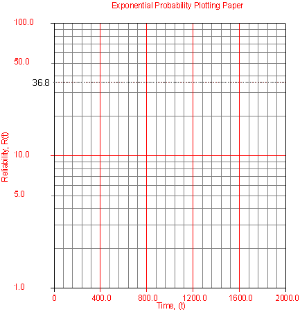
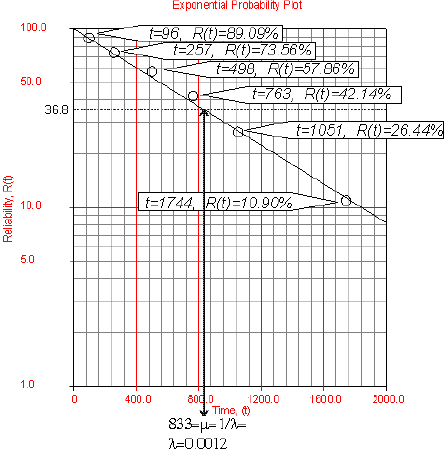
- • On an exponential probability paper, plot the times on the x-axis and their corresponding
rank value on the y-axis. Fig. 4 displays an example of an exponential probability paper. The
paper is simply a log-linear paper. (The solution is given in Fig. 2.)
- • Draw the best possible straight line that goes through the [math]\displaystyle{ t=0 }[/math] and [math]\displaystyle{ (t)=100% }[/math] point and through the plotted points (as shown in Fig. 5).
- • At the [math]\displaystyle{ Q(t)=63.2% }[/math] or [math]\displaystyle{ R(t)=36.8% }[/math] ordinate point, draw a
straight horizontal line until this line intersects the fitted straight line. Draw a vertical line through this intersection until it crosses the abscissa. The value at the intersection of the abscissa is the estimate of the mean. For this case, [math]\displaystyle{ \widehat{\mu }=833 }[/math] hr which means that [math]\displaystyle{ \lambda =\tfrac{1}{\mu }=0.0012 }[/math] . (This is always at 63.2% since [math]\displaystyle{ (T)=1-{{e}^{-\tfrac{\mu }{\mu }}}=1-{{e}^{-1}}=0.632=63.2%). }[/math]
Now any reliability value for any mission time [math]\displaystyle{ t }[/math] can be obtained. For example, the
reliability for a mission of 15 hr, or any other time, can now be obtained either from the plot or analytically (i.e. using the equations given in Section [math]\displaystyle{ 5.1.1 }[/math] ).
To obtain the value from the plot, draw a vertical line from the abscissa, at [math]\displaystyle{ t=15 }[/math]
hr, to the fitted line. Draw a horizontal line from this intersection to the ordinate and read
[math]\displaystyle{ R(t) }[/math] . In this case, [math]\displaystyle{ R(t=15)=98.15% }[/math] . This can also be obtained
analytically, from the exponential reliability function.
MLE Parameter Estimation
The parameter of the exponential distribution can also be estimated using the maximum likelihood estimation (MLE) method. This log-likelihood function is:
- [math]\displaystyle{ \ln (L)=\Lambda =\underset{i=1}{\overset{{{F}_{e}}}{\mathop \sum }}\,{{N}_{i}}\ln \left[ \lambda {{e}^{-\lambda {{T}_{i}}}} \right]-\underset{i=1}{\overset{S}{\mathop \sum }}\,N_{i}^{\prime }\lambda T_{i}^{\prime }+\overset{FI}{\mathop{\underset{i=1}{\mathop{\underset{}{\overset{}{\mathop \sum }}\,}}\,}}\,N_{i}^{\prime \prime }\ln [R_{Li}^{\prime \prime }-R_{Ri}^{\prime \prime }] }[/math]
where:
- [math]\displaystyle{ R_{Li}^{\prime \prime }={{e}^{-\lambda T_{Li}^{\prime \prime }}} }[/math]
- [math]\displaystyle{ R_{Ri}^{\prime \prime }={{e}^{-\lambda T_{Ri}^{\prime \prime }}} }[/math]
and
- • [math]\displaystyle{ {{F}_{e}} }[/math] is the number of groups of times-to-failure data points.
- • [math]\displaystyle{ {{N}_{i}} }[/math] is the number of times-to-failure in the [math]\displaystyle{ {{i}^{th}} }[/math] time-to-failure data group.
- • [math]\displaystyle{ \lambda }[/math] is the failure rate parameter (unknown a priori, the only parameter to be found).
- • [math]\displaystyle{ {{T}_{i}} }[/math] is the time of the [math]\displaystyle{ {{i}^{th}} }[/math] group of time-to-failure data.
- • [math]\displaystyle{ S }[/math] is the number of groups of suspension data points.
- • [math]\displaystyle{ N_{i}^{\prime } }[/math] is the number of suspensions in the [math]\displaystyle{ {{i}^{th}} }[/math] group of suspension data points.
- • [math]\displaystyle{ T_{i}^{\prime } }[/math] is the time of the [math]\displaystyle{ {{i}^{th}} }[/math] suspension data group.
- • [math]\displaystyle{ FI }[/math] is the number of interval data groups.
- • [math]\displaystyle{ N_{i}^{\prime \prime } }[/math] is the number of intervals in the i [math]\displaystyle{ ^{th} }[/math] group of data intervals.
- • [math]\displaystyle{ T_{Li}^{\prime \prime } }[/math] is the beginning of the i [math]\displaystyle{ ^{th} }[/math] interval.
- • [math]\displaystyle{ T_{Ri}^{\prime \prime } }[/math] is the ending of the i [math]\displaystyle{ ^{th} }[/math] interval.
The solution will be found by solving for a parameter [math]\displaystyle{ \widehat{\lambda } }[/math] so that [math]\displaystyle{ \tfrac{\partial \Lambda }{\partial \lambda }=0 }[/math] where:
- [math]\displaystyle{ \frac{\partial \Lambda }{\partial \lambda }=\underset{i=1}{\overset{{{F}_{e}}}{\mathop \sum }}\,{{N}_{i}}\left( \frac{1}{\lambda }-{{T}_{i}} \right)-\underset{i=1}{\overset{S}{\mathop \sum }}\,N_{i}^{\prime }T_{i}^{\prime }-\overset{FI}{\mathop{\underset{i=1}{\mathop{\underset{}{\overset{}{\mathop \sum }}\,}}\,}}\,N_{i}^{\prime \prime }\frac{T_{Li}^{\prime \prime }R_{Li}^{\prime \prime }-T_{Ri}^{\prime \prime }R_{Ri}^{\prime \prime }}{R_{Li}^{\prime \prime }-R_{Ri}^{\prime \prime }} }[/math]
Example 2
Using the same data as in the probability plotting example (Example 1), and assuming an exponential distribution, estimate the parameter using the MLE method.
Solution
In this example we have non-grouped data without suspensions. Thus Eqn. (exp-mle) becomes:
- [math]\displaystyle{ \frac{\partial \Lambda }{\partial \lambda }=\underset{i=1}{\overset{{{F}_{e}}}{\mathop \sum }}\,\left[ \frac{1}{\lambda }-\left( {{T}_{i}} \right) \right]=\underset{i=1}{\overset{14}{\mathop \sum }}\,\left[ \frac{1}{\lambda }-\left( {{T}_{i}} \right) \right]=0 }[/math]
Substituting the values for [math]\displaystyle{ T }[/math] we get:
- [math]\displaystyle{ \begin{align} \frac{6}{\lambda }= & 4409,\text{ or:} \\ \lambda = & 0.00136\text{ failure/hr} \end{align} }[/math]

