Lloyd-Lipow

Lloyd-Lipow

Lloyd and Lipow (1962) considered a situation in which a test program is conducted in [math]\displaystyle{ N }[/math] stages. Each stage consists of a certain number of trials of an item undergoing testing and the data set is recorded as successes or failures. All tests in a given stage of testing involve similar items. The results of each stage of testing are used to improve the item for further testing in the next stage. For the [math]\displaystyle{ {{k}^{th}} }[/math] group of data, taken in chronological order, there are [math]\displaystyle{ {{n}_{k}} }[/math] tests with [math]\displaystyle{ {{S}_{k}} }[/math] observed successes. The reliability growth function is then [6]:

[math]\displaystyle{ {{R}_{k}}={{R}_{\infty }}-\frac{\alpha }{k} }[/math]

where:

[math]\displaystyle{ \begin{align} & {{R}_{k}}= & \text{ the actual reliability during the }{{k}^{th}}\text{ stage of testing} \\ & {{R}_{\infty }}= & \text{ the ultimate reliability attained if }k\to \infty \\ & \alpha \gt 0= & \text{modifies the rate of growth} \end{align} }[/math]

Note that essentially, [math]\displaystyle{ {{R}_{k}}=\tfrac{{{S}_{k}}}{{{n}_{k}}} }[/math] . If the data set consists of reliability data, then [math]\displaystyle{ {{S}_{k}} }[/math] is assumed to be the observed reliability given and [math]\displaystyle{ {{n}_{k}} }[/math] is considered 1.

Parameter Estimation

When analyzing reliability data in RGA, you have the option to enter the reliability values in percent or in decimal format. However, [math]\displaystyle{ {{\hat{R}}_{\infty }} }[/math] will always be returned in decimal format and not in percent. The estimated parameters in RGA are unitless.

Maximum Likelihood Estimators

For the [math]\displaystyle{ {{k}^{th}} }[/math] stage:

[math]\displaystyle{ {{L}_{k}}=const.\text{ }R_{k}^{{{S}_{k}}}{{(1-{{R}_{k}})}^{{{n}_{k}}-{{S}_{k}}}} }[/math]

And assuming that the results are independent between stages:

[math]\displaystyle{ L=\underset{k=1}{\overset{N}{\mathop \prod }}\,R_{k}^{{{S}_{k}}}{{(1-{{R}_{k}})}^{{{n}_{k}}-{{S}_{k}}}} }[/math]

Then taking the natural log gives:

[math]\displaystyle{ \Lambda =\underset{k=1}{\overset{N}{\mathop \sum }}\,{{S}_{k}}\ln \left( {{R}_{\infty }}-\frac{\alpha }{k} \right)+\underset{k=1}{\overset{N}{\mathop \sum }}\,({{n}_{k}}-{{S}_{k}})\ln \left( 1-{{R}_{\infty }}+\frac{\alpha }{k} \right) }[/math]

Differentiating with respect to [math]\displaystyle{ {{R}_{\infty }} }[/math] and [math]\displaystyle{ \alpha , }[/math] yields:

[math]\displaystyle{ \frac{\partial \Lambda }{\partial {{R}_{\infty }}}=\underset{k=1}{\overset{N}{\mathop \sum }}\,\frac{{{S}_{k}}}{{{R}_{\infty }}-\tfrac{\alpha }{k}}-\underset{k=1}{\overset{N}{\mathop \sum }}\,\frac{{{n}_{k}}-{{S}_{k}}}{1-{{R}_{\infty }}+\tfrac{\alpha }{k}} }[/math]

[math]\displaystyle{ \frac{\partial \Lambda }{\partial \alpha }=-\underset{k=1}{\overset{N}{\mathop \sum }}\,\frac{\tfrac{{{S}_{k}}}{k}}{{{R}_{\infty }}-\tfrac{\alpha }{k}}+\underset{k=1}{\overset{N}{\mathop \sum }}\,\frac{\tfrac{{{n}_{k}}-{{S}_{k}}}{k}}{1-{{R}_{\infty }}+\tfrac{\alpha }{k}} }[/math]

Rearranging Eqns. (R1) and (alpha1) and setting equal to zero gives:

[math]\displaystyle{ \frac{\partial \Lambda }{\partial {{R}_{\infty }}}=\underset{k=1}{\overset{N}{\mathop \sum }}\,\frac{\tfrac{{{S}_{k}}}{{{n}_{k}}}-\left( {{R}_{\infty }}-\tfrac{\alpha }{k} \right)}{\tfrac{1}{{{n}_{k}}}\left( {{R}_{\infty }}-\tfrac{\alpha }{k} \right)\left( 1-{{R}_{\infty }}+\tfrac{\alpha }{k} \right)}=0 }[/math]

[math]\displaystyle{ \frac{\partial \Lambda }{\partial \alpha }=-\underset{k=1}{\overset{N}{\mathop \sum }}\,\frac{\tfrac{1}{k}\tfrac{{{S}_{k}}}{{{n}_{k}}}-\left( {{R}_{\infty }}-\tfrac{\alpha }{k} \right)\tfrac{1}{k}}{\tfrac{1}{{{n}_{k}}}\left( {{R}_{\infty }}-\tfrac{\alpha }{k} \right)\left( 1-{{R}_{\infty }}+\tfrac{\alpha }{k} \right)}=0 }[/math]

Eqns. (R2) and (alpha2) can be solved simultaneously for [math]\displaystyle{ \widehat{\alpha } }[/math] and [math]\displaystyle{ {{\hat{R}}_{\infty }} }[/math] . It should be noted that a closed form solution does not exist for either of the parameters; thus they must be estimated numerically.

Least Squares Estimators

To obtain least squares estimators for [math]\displaystyle{ {{R}_{\infty }} }[/math] and [math]\displaystyle{ \alpha }[/math] , the sum of squares, [math]\displaystyle{ Q }[/math] , of the deviations of the observed success-ratio, [math]\displaystyle{ {{S}_{k}}/{{n}_{k}} }[/math] , is minimized from its expected value, [math]\displaystyle{ {{R}_{\infty }}-\tfrac{\alpha }{k} }[/math] , with respect to the parameters [math]\displaystyle{ {{R}_{\infty }} }[/math] and [math]\displaystyle{ \alpha . }[/math] Therefore, [math]\displaystyle{ Q }[/math] is expressed as:

[math]\displaystyle{ Q=\underset{k=1}{\overset{N}{\mathop \sum }}\,{{\left( \frac{{{S}_{k}}}{{{n}_{k}}}-{{R}_{\infty }}+\frac{\alpha }{k} \right)}^{2}} }[/math]

Taking the derivatives with respect to [math]\displaystyle{ {{R}_{\infty }} }[/math] and [math]\displaystyle{ \alpha }[/math] and setting equal to zero yields:

[math]\displaystyle{ \begin{align} & \frac{\partial Q}{\partial {{R}_{\infty }}}= & -2\underset{k=1}{\overset{N}{\mathop \sum }}\,\left( \frac{{{S}_{k}}}{{{n}_{k}}}-{{R}_{\infty }}+\frac{\alpha }{k} \right)=0 \\ & \frac{\partial Q}{\partial \alpha }= & 2\underset{k=1}{\overset{N}{\mathop \sum }}\,\left( \frac{{{S}_{k}}}{{{n}_{k}}}-{{R}_{\infty }}+\frac{\alpha }{k} \right)\frac{1}{k}=0 \end{align} }[/math]

Solving Eqns. (pqprll) and (pqpall) simultaneously, the least squares estimates of [math]\displaystyle{ {{R}_{\infty }} }[/math] and [math]\displaystyle{ \alpha }[/math] are:

[math]\displaystyle{ {{\hat{R}}_{\infty }}=\frac{\underset{k=1}{\overset{N}{\mathop{\sum }}}\,\tfrac{1}{{{k}^{2}}}\underset{k=1}{\overset{N}{\mathop{\sum }}}\,\tfrac{{{S}_{k}}}{{{n}_{k}}}-\underset{k=1}{\overset{N}{\mathop{\sum }}}\,\tfrac{1}{k}\underset{k=1}{\overset{N}{\mathop{\sum }}}\,\tfrac{{{S}_{k}}}{k{{n}_{k}}}}{N\underset{k=1}{\overset{N}{\mathop{\sum }}}\,\tfrac{1}{{{k}^{2}}}-{{\left( \underset{k=1}{\overset{N}{\mathop{\sum }}}\,\tfrac{1}{k} \right)}^{2}}} }[/math]

or:

[math]\displaystyle{ \text{ }{{\hat{R}}_{\infty }}=\frac{\underset{k=1}{\overset{N}{\mathop{\sum }}}\,\tfrac{1}{{{k}^{2}}}\underset{k=1}{\overset{N}{\mathop{\sum }}}\,{{R}_{k}}-\underset{k=1}{\overset{N}{\mathop{\sum }}}\,\tfrac{1}{k}\underset{k=1}{\overset{N}{\mathop{\sum }}}\,\tfrac{{{R}_{k}}}{k}}{N\underset{k=1}{\overset{N}{\mathop{\sum }}}\,\tfrac{1}{{{k}^{2}}}-{{\left( \underset{k=1}{\overset{N}{\mathop{\sum }}}\,\tfrac{1}{k} \right)}^{2}}} }[/math]

and:

[math]\displaystyle{ \hat{\alpha }=\frac{\underset{k=1}{\overset{N}{\mathop{\sum }}}\,\tfrac{1}{k}\underset{k=1}{\overset{N}{\mathop{\sum }}}\,\tfrac{{{S}_{k}}}{{{n}_{k}}}-N\underset{k=1}{\overset{N}{\mathop{\sum }}}\,\tfrac{{{S}_{k}}}{k{{n}_{k}}}}{N\underset{k=1}{\overset{N}{\mathop{\sum }}}\,\tfrac{1}{{{k}^{2}}}-{{\left( \underset{k=1}{\overset{N}{\mathop{\sum }}}\,\tfrac{1}{k} \right)}^{2}}} }[/math]

or:

[math]\displaystyle{ \hat{\alpha }=\frac{\underset{k=1}{\overset{N}{\mathop{\sum }}}\,\tfrac{1}{k}\underset{k=1}{\overset{N}{\mathop{\sum }}}\,{{R}_{k}}-N\underset{k=1}{\overset{N}{\mathop{\sum }}}\,\tfrac{{{R}_{k}}}{k}}{N\underset{k=1}{\overset{N}{\mathop{\sum }}}\,\tfrac{1}{{{k}^{2}}}-{{\left( \underset{k=1}{\overset{N}{\mathop{\sum }}}\,\tfrac{1}{k} \right)}^{2}}} }[/math]

Example 1
After a 20-stage reliability development test program, 20 groups of success/failure data were obtained and are given in Table 6.1. Do the following:
1) Fit the Lloyd-Lipow model to the data using least squares.
2) Plot the reliabilities predicted by the Lloyd-Lipow model along with the observed reliabilities and compare the results.

Table 6.1 - The test results and reliabilities of each stage calculated from raw data and the predicted reliability

Test Stage Number([math]\displaystyle{ k }[/math])	Number of Tests in Stage([math]\displaystyle{ n_k }[/math])	Number of Successful Tests([math]\displaystyle{ S_k }[/math])	Raw Data Reliability	Lloyd-Lipow Reliability
1	9	6	0.667	0.7002
2	9	5	0.556	0.7369
3	8	7	0.875	0.7552
4	10	6	0.600	0.7662
5	9	7	0.778	0.7736
6	10	8	0.800	0.7788
7	10	7	0.700	0.7827
8	10	6	0.600	0.7858
9	11	7	0.636	0.7882
10	11	9	0.818	0.7902
11	9	9	1.000	0.7919
12	12	10	0.833	0.7933
13	12	9	0.750	0.7945
14	11	8	0.727	0.7956
15	10	7	0.700	0.7965
16	10	8	0.800	0.7973
17	11	10	0.909	0.7980
18	10	9	0.900	0.7987
19	9	8	0.889	0.7992
20	8	7	0.875	0.7998

Solution
From Table 6.1, the least squares estimates are:

[math]\displaystyle{ \begin{align} & \underset{k=1}{\overset{N}{\mathop \sum }}\,\frac{1}{k}= & \underset{k=1}{\overset{20}{\mathop \sum }}\,\frac{1}{k}=3.5977 \\ & \underset{k=1}{\overset{N}{\mathop \sum }}\,\frac{1}{{{k}^{2}}}= & \underset{k=1}{\overset{20}{\mathop \sum }}\,\frac{1}{{{k}^{2}}}=1.5962 \\ & \underset{k=1}{\overset{N}{\mathop \sum }}\,\frac{{{S}_{k}}}{{{n}_{k}}}= & \underset{k=1}{\overset{20}{\mathop \sum }}\,\frac{{{S}_{k}}}{{{n}_{k}}}=15.4131 \end{align} }[/math]

and:

[math]\displaystyle{ \underset{k=1}{\overset{N}{\mathop \sum }}\,\frac{{{S}_{k}}}{k\cdot {{n}_{k}}}=\underset{k=1}{\overset{20}{\mathop \sum }}\,\frac{{{S}_{k}}}{k\cdot {{n}_{k}}}=2.5632 }[/math]

Substituting into Eqns. (ar) and (alph) yields:

[math]\displaystyle{ \begin{align} & {{{\hat{R}}}_{\infty }}= & \frac{(1.5962)(15.413)-(3.5977)(2.5637)}{(20)(1.5962)-{{(3.5977)}^{2}}} \\ & = & 0.8104 \end{align} }[/math]

and:

[math]\displaystyle{ \begin{align} & \hat{\alpha }= & \frac{(3.5977)(15.413)-(20)(2.5637)}{(20)(1.5962)-{{(3.5977)}^{2}}} \\ & = & 0.2207 \end{align} }[/math]

Therefore, the Lloyd-Lipow reliability growth model is as follows, where [math]\displaystyle{ k }[/math] is the test stage.

[math]\displaystyle{ {{R}_{k}}=0.8104-\frac{0.2201}{k} }[/math]

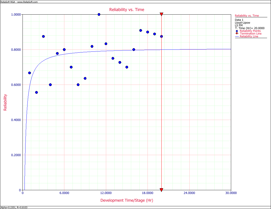
The reliabilities from the raw data and the reliabilities predicted from Eqn. (eq33) are given in the last two columns of Table 6.1. Figure llfig61 shows the plot. Based on the given data, the model cannot do much more than to basically fit a line through the middle of the points.

[math]\displaystyle{ }[/math]

Figure 6.1: Comparison of the predicted reliability and the raw data.

Confidence Bounds

In this section, the methods used in RGA to estimate the confidence bounds under the Lloyd-Lipow model will be presented. One of the properties of maximum likelihood estimators is that they are asymptotically normal. This indicates that they are normally distributed for large samples [6][7]. Additionally, since the parameter [math]\displaystyle{ \alpha }[/math] must be positive, [math]\displaystyle{ \ln \alpha }[/math] is treated as being normally distributed as well. The parameter [math]\displaystyle{ {{R}_{\infty }} }[/math] represents the ultimate reliability that would be attained if [math]\displaystyle{ k\to \infty }[/math] . [math]\displaystyle{ {{R}_{k}} }[/math] is the actual reliability during the [math]\displaystyle{ {{k}^{th}} }[/math] stage of testing. Therefore, [math]\displaystyle{ {{R}_{\infty }} }[/math] and [math]\displaystyle{ {{R}_{k}} }[/math] will be between 0 and 1. Consequently, the endpoints of the confidence intervals of the parameters [math]\displaystyle{ {{R}_{\infty }} }[/math] and [math]\displaystyle{ {{R}_{k}} }[/math] also will be between 0 and 1. To obtain the confidence interval, it is common practice to use the logit transformation. The confidence bounds on the parameters [math]\displaystyle{ \alpha }[/math] and [math]\displaystyle{ {{R}_{\infty }} }[/math] are given by:

[math]\displaystyle{ C{{B}_{\alpha }}=\hat{\alpha }{{e}^{\pm {{z}_{\alpha /2}}\sqrt{Var(\hat{\alpha })}/\hat{\alpha }}} }[/math]

[math]\displaystyle{ C{{B}_{{{R}_{\infty }}}}=\frac{{{{\hat{R}}}_{\infty }}}{{{{\hat{R}}}_{\infty }}+(1-{{{\hat{R}}}_{\infty }}){{e}^{\pm {{z}_{\alpha /2}}\sqrt{Var({{{\hat{R}}}_{\infty }})}/\left[ {{{\hat{R}}}_{\infty }}(1-{{{\hat{R}}}_{\infty }}) \right]}}} }[/math]

where [math]\displaystyle{ {{z}_{\alpha /2}} }[/math] represents the percentage points of the [math]\displaystyle{ N(0,1) }[/math] distribution such that [math]\displaystyle{ P\{z\ge {{z}_{\alpha /2}}\}=\alpha /2 }[/math] . The confidence bounds on reliability are given by:

[math]\displaystyle{ CB=\frac{{{{\hat{R}}}_{k}}}{{{{\hat{R}}}_{k}}+(1-{{{\hat{R}}}_{k}}){{e}^{\pm {{z}_{\alpha /2}}\sqrt{Var({{{\hat{R}}}_{k}})}/\left[ {{{\hat{R}}}_{k}}(1-{{{\hat{R}}}_{k}}) \right]}}} }[/math]

where:

[math]\displaystyle{ Var({{\widehat{R}}_{k}})=Var({{\widehat{R}}_{\infty }})+\frac{1}{{{k}^{2}}}\cdot Var(\widehat{\alpha })-\frac{2}{k}\cdot Cov({{\widehat{R}}_{\infty }},\widehat{\alpha }) }[/math]

All the variances can be calculated using the Fisher Matrix:

[math]\displaystyle{ {{\left[ \begin{matrix} -\tfrac{{{\partial }^{2}}\Lambda }{\partial R_{\infty }^{2}} & -\tfrac{{{\partial }^{2}}\Lambda }{\partial \alpha \partial {{R}_{\infty }}} \\ -\tfrac{{{\partial }^{2}}\Lambda }{\partial \alpha \partial {{R}_{\infty }}} & -\tfrac{{{\partial }^{2}}\Lambda }{\partial {{\alpha }^{2}}} \\ \end{matrix} \right]}^{-1}}=\left[ \begin{matrix} Var({{\widehat{R}}_{\infty }}) & Cov({{\widehat{R}}_{\infty }},\widehat{\alpha }) \\ Cov({{\widehat{R}}_{\infty }},\widehat{\alpha }) & Var(\widehat{\alpha }) \\ \end{matrix} \right] }[/math]

From Eqns. (R2) and (alpha2), taking the second partial derivatives yields:

[math]\displaystyle{ \frac{{{\partial }^{2}}\Lambda }{\partial R_{\infty }^{2}}=-\underset{k=1}{\overset{N}{\mathop \sum }}\,\frac{{{S}_{k}}}{{{\left( {{R}_{\infty }}-\tfrac{\alpha }{k} \right)}^{2}}}-\underset{k=1}{\overset{N}{\mathop \sum }}\,\frac{{{n}_{k}}-{{S}_{k}}}{{{\left( 1-{{R}_{\infty }}+\tfrac{\alpha }{k} \right)}^{2}}} }[/math]

[math]\displaystyle{ \frac{{{\partial }^{2}}\Lambda }{\partial {{\alpha }^{2}}}=-\underset{k=1}{\overset{N}{\mathop \sum }}\,\frac{\tfrac{{{S}_{k}}}{{{k}^{2}}}}{{{\left( {{R}_{\infty }}-\tfrac{\alpha }{k} \right)}^{2}}}-\underset{k=1}{\overset{N}{\mathop \sum }}\,\frac{\tfrac{{{n}_{k}}-{{S}_{k}}}{{{k}^{2}}}}{{{\left( 1-{{R}_{\infty }}+\tfrac{\alpha }{k} \right)}^{2}}} }[/math]

and:

[math]\displaystyle{ \frac{{{\partial }^{2}}\Lambda }{\partial {{R}_{\infty }}\partial \alpha }=\underset{k=1}{\overset{N}{\mathop \sum }}\,\frac{\tfrac{{{S}_{k}}}{k}}{{{\left( {{R}_{\infty }}-\tfrac{\alpha }{k} \right)}^{2}}}-\underset{k=1}{\overset{N}{\mathop \sum }}\,\frac{\tfrac{{{n}_{k}}-{{S}_{k}}}{k}}{{{\left( 1-{{R}_{\infty }}+\tfrac{\alpha }{k} \right)}^{2}}} }[/math]

Now the confidence bounds can be obtained after calculating Eqns. (cbll2) through (cbll5) and substituting into the Fisher Matrix.


Example 2
Plot the confidence bounds for the data in Table 6.1.


Solution
From Eqns. (cbll3), (cbll4) and (cbll5):

[math]\displaystyle{ \begin{align} & \frac{{{\partial }^{2}}\Lambda }{\partial R_{\infty }^{2}}= & -255.3835-937.2902=-1192.6737 \\ & \frac{{{\partial }^{2}}\Lambda }{\partial {{\alpha }^{2}}}= & -24.4575-43.3930=-67.8505 \\ & \frac{{{\partial }^{2}}\Lambda }{\partial {{R}_{\infty }}\partial \alpha }= & 48.6606-140.7518=-92.0912 \end{align} }[/math]

The variances can be calculated using the Fisher Matrix:

[math]\displaystyle{ \begin{align} & {{\left[ \begin{matrix} 1192.6737 & 92.0912 \\ 92.0912 & 67.8505 \\ \end{matrix} \right]}^{-1}}= & \left[ \begin{matrix} Var({{\widehat{R}}_{\infty }}) & Cov({{\widehat{R}}_{\infty }},\widehat{\alpha }) \\ Cov({{\widehat{R}}_{\infty }},\widehat{\alpha }) & Var(\widehat{\alpha }) \\ \end{matrix} \right] \\ & = & \left[ \begin{matrix} 0.00093661 & -0.00127123 \\ -0.00127123 & 0.01646371 \\ \end{matrix} \right] \end{align} }[/math]

[math]\displaystyle{ }[/math]

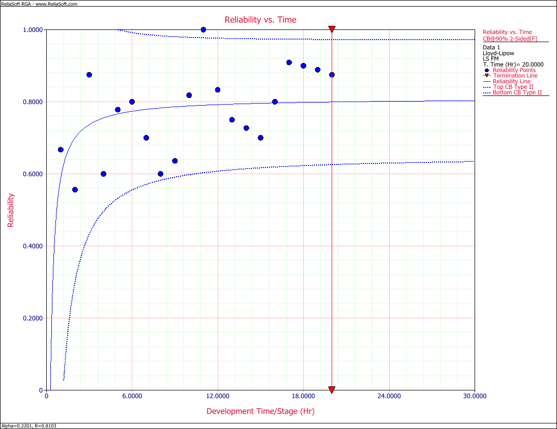
Figure 6.2: Predicted reliability with 90% confidence bounds.

The variance of [math]\displaystyle{ {{R}_{k}} }[/math] is obtained from Eqn. (cbll2) such that:

[math]\displaystyle{ Var({{\widehat{R}}_{k}})=0.00093661+\frac{1}{{{k}^{2}}}\cdot 0.01646371+\frac{2}{k}\cdot 0.00127123 }[/math]

Now Eqn. (llrc) can be calculated and the associated confidence bounds at the [math]\displaystyle{ 90% }[/math] confidence level are plotted in Figure llfig62 with the predicted reliability, [math]\displaystyle{ {{R}_{k}} }[/math] .


Example 3
Consider the success/failure data given in Table 6.2. Solve for the Lloyd-Lipow parameters using least squares analysis and plot the Lloyd-Lipow reliability with 2-sided confidence bounds at the 90% confidence level.

Table 6.2 - Success/failure data for a variable number

of tests performed in each test stage

Test Stage Number([math]\displaystyle{ k }[/math])	Result	Number of Tests([math]\displaystyle{ n_k }[/math]>	Successful Tests([math]\displaystyle{ S_k=R_i }[/math])
1	F	1	0
2	F	1	0
3	F	1	0
4	S	1	0.2500
5	F	1	0.2000
6	F	1	0.1667
7	S	1	0.2857
8	S	1	0.3750
9	S	1	0.4444
10	S	1	0.5000
11	S	1	0.5455
12	S	1	0.5833
13	S	1	0.6154
14	S	1	0.6429
15	S	1	0.6667
16	S	1	0.6875
17	F	1	0.6471
18	S	1	0.6667
19	F	1	0.6316
20	S	1	0.6500
21	S	1	0.6667
22	S	1	0.6818

Solution
Note that the data set contains three consecutive failures at the beginning of the test. These failures will be ignored throughout the analysis because it is considered that the test starts when the reliability is not equal to zero or one. The number of data points is now reduced to 19. Also note that the only time that the first three first failures are considered is to calculate the observed reliability in the test. For example, given this data set, the observed reliability at stage 4 is [math]\displaystyle{ 1/4=0.25 }[/math] . This is considered to be the reliability at stage 1.
From Table 6.2, the least squares estimates can be calculated as follows:

[math]\displaystyle{ \begin{align} & \underset{k=1}{\overset{N}{\mathop \sum }}\,\frac{1}{k}= & \underset{k=1}{\overset{19}{\mathop \sum }}\,\frac{1}{k}=3.54774 \\ & \underset{k=1}{\overset{N}{\mathop \sum }}\,\frac{1}{{{k}^{2}}}= & \underset{k=1}{\overset{19}{\mathop \sum }}\,\frac{1}{{{k}^{2}}}=1.5936 \\ & \underset{k=1}{\overset{N}{\mathop \sum }}\,\frac{{{S}_{k}}}{{{n}_{k}}}= & \underset{k=1}{\overset{19}{\mathop \sum }}\,\frac{{{S}_{k}}}{{{n}_{k}}}=9.907 \end{align} }[/math]

and:

[math]\displaystyle{ \underset{k=1}{\overset{N}{\mathop \sum }}\,\frac{{{S}_{k}}}{k\cdot {{n}_{k}}}=\underset{k=1}{\overset{19}{\mathop \sum }}\,\frac{{{S}_{k}}}{k\cdot {{n}_{k}}}=1.3002 }[/math]

Substituting into Eqns. (ar) and (alph) yields:

[math]\displaystyle{ \begin{align} & {{{\hat{R}}}_{\infty }}= & \frac{(1.5936)(9.907)-(3.5477)(1.3002)}{(19)(1.5936)-{{(3.5477)}^{2}}} \\ & = & 0.6316 \end{align} }[/math]

and:

[math]\displaystyle{ \begin{align} & \hat{\alpha }= & \frac{(3.5477)(9.907)-(19)(1.3002)}{(19)(1.5936)-{{(3.5477)}^{2}}} \\ & = & 0.5902 \end{align} }[/math]

Therefore, the Lloyd-Lipow reliability growth model is as follows, where [math]\displaystyle{ k }[/math] is the number of the test stage.

[math]\displaystyle{ {{R}_{k}}=0.6316-\frac{0.5902}{k} }[/math]

From Eqns. (cbll3), (cbll4), (cbll5) and the data given in Table 6.2:

[math]\displaystyle{ \begin{align} & \frac{{{\partial }^{2}}\Lambda }{\partial R_{\infty }^{2}}= & -176.847-40.500=-217.347 \\ & \frac{{{\partial }^{2}}\Lambda }{\partial {{\alpha }^{2}}}= & -146.763-2.1274=-148.891 \\ & \frac{{{\partial }^{2}}\Lambda }{\partial {{R}_{\infty }}\partial \alpha }= & 149.909-6.5660=143.343 \end{align} }[/math]

The variances can be calculated using the Fisher Matrix:

[math]\displaystyle{ \begin{align} & {{\left[ \begin{matrix} 217.347 & -143.343 \\ -143.343 & 148.891 \\ \end{matrix} \right]}^{-1}}= & \left[ \begin{matrix} Var({{\widehat{R}}_{\infty }}) & Cov({{\widehat{R}}_{\infty }},\widehat{\alpha }) \\ Cov({{\widehat{R}}_{\infty }},\widehat{\alpha }) & Var(\widehat{\alpha }) \\ \end{matrix} \right] \\ & = & \left[ \begin{matrix} 0.0126033 & 0.0121335 \\ 0.0121335 & 0.0183977 \\ \end{matrix} \right] \end{align} }[/math]

The variance of [math]\displaystyle{ {{R}_{k}} }[/math] is obtained from Eqn. (cbll2):

[math]\displaystyle{ Var({{\widehat{R}}_{k}})=0.0126031+\frac{1}{{{k}^{2}}}\cdot 0.0183977-\frac{2}{k}\cdot 0.0121335 }[/math]

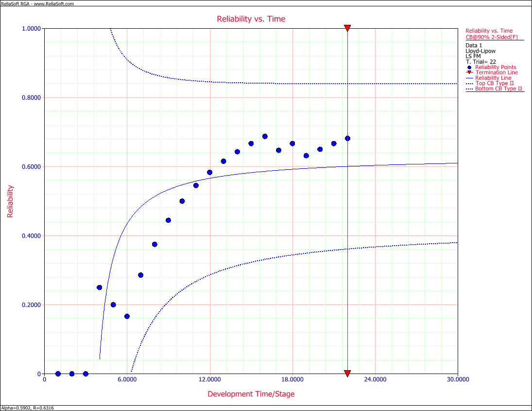
Now Eqn. (llrc) can be calculated and the associated confidence bounds on reliability at the [math]\displaystyle{ 90% }[/math] confidence level are plotted in Figure llfig63 with the predicted reliability, [math]\displaystyle{ {{R}_{k}} }[/math] .

[math]\displaystyle{ }[/math]

Figure 6.3: Reliability vs. Time Plot with 90% confidence bounds.

General Examples

Example 4

A 15-stage reliability development test program was performed. The grouped per configuration data set that was obtained is given in Table 6.3. Do the following:

1) Fit the Lloyd-Lipow model to the data using MLE.
2) What is the maximum reliability attained as the number of test stages approaches infinity?
3) What is the maximum achievable reliability with a 90% confidence level?

Table 6.3 - Grouped per Configuration data for Example 4

Stage, [math]\displaystyle{ k }[/math]	Number of Tests ([math]\displaystyle{ n_k }[/math])	Number of Successes ([math]\displaystyle{ S_k }[/math])
1	10	3
2	10	3
3	10	4
4	10	5
5	10	5
6	12	6
7	12	5
8	12	7
9	14	8
10	14	8
11	14	10
12	14	12
13	14	11
14	14	12
15	14	12

Solution to Example 4

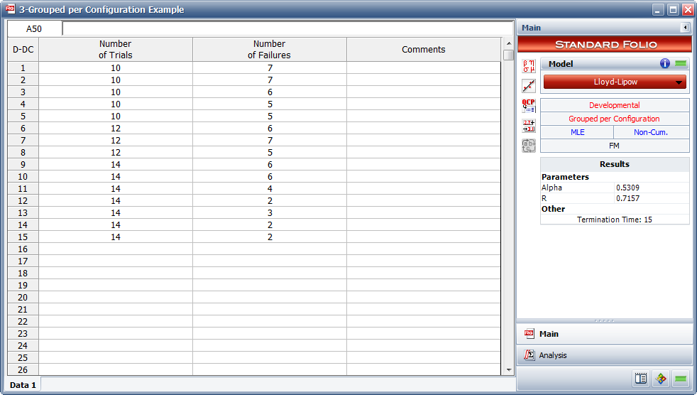
1) Figure figLLSe11 displays the entered data and the estimated Lloyd-Lipow parameters.
2) The maximum achievable reliability as the number of test stages approaches infinity is equal to the value of [math]\displaystyle{ R }[/math] . Therefore, [math]\displaystyle{ R=0.7157 }[/math] .
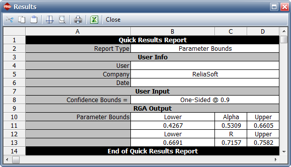
3) The maximum achievable reliability with a 90% confidence level can be estimated by viewing the confidence bounds on the parameters in the QCP, as shown in Figure QCPex4. The lower bound on the value of [math]\displaystyle{ R }[/math] is equal to [math]\displaystyle{ 0.6691 }[/math] .

[math]\displaystyle{ }[/math]

Figure 6.4: Estimated Lloyd-Lipow parameters using MLE.

Figure 6.5: Confidence bounds on the parameters.

Example 5

Given the reliability data in Table 6.4, do the following:

1) Fit the Lloyd-Lipow model to the data using least squares analysis.
2) Plot the Lloyd-Lipow reliability with 90% 2-sided confidence bounds.
3) Determine how many months of testing are required to achieve a reliability goal of 90%.
4) Determine what is the attainable reliability if the maximum duration of testing is 30 months.

Table 6.4 - Reliability data

Time(months)	Reliability(%)
1	33.35
2	42.50
3	58.02
4	68.50
5	74.20
6	80.00
7	82.30
8	89.50
9	91.00
10	92.10

Solution to Example 5

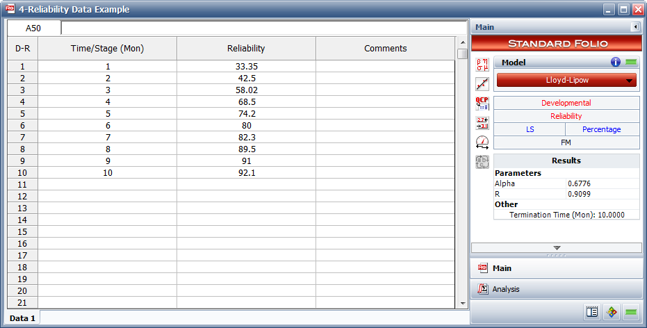
1) Figure figLLSe21 displays the estimated parameters.
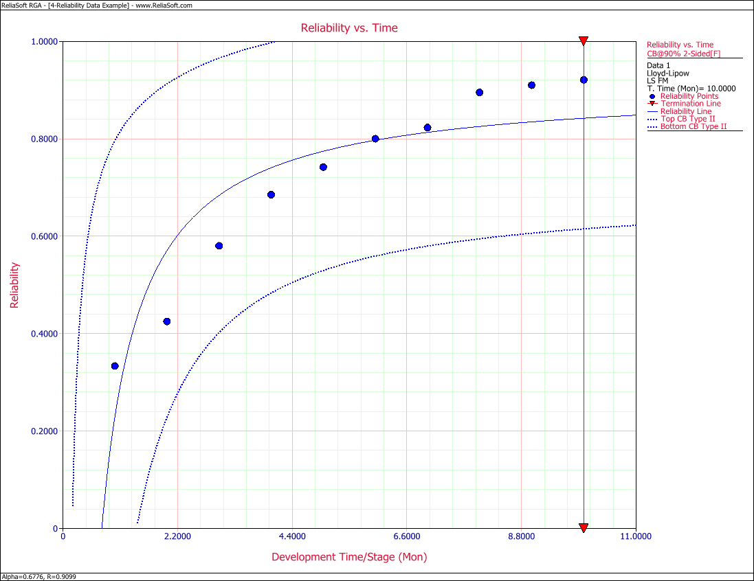
2) Figure figLLSe22 displays Reliability vs. Time plot with 90% 2-sided confidence bounds.
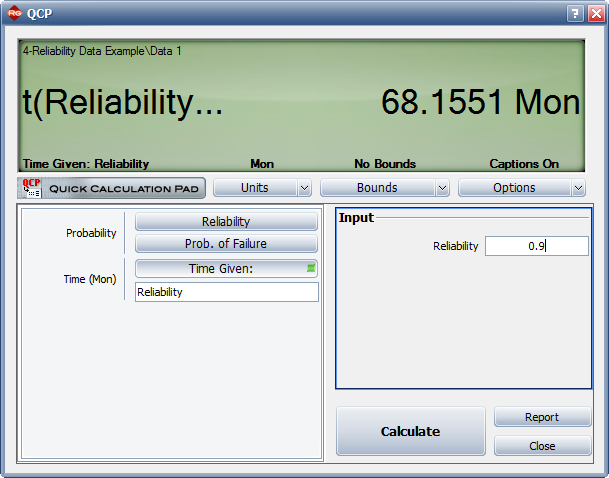
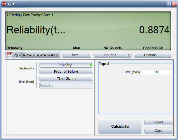
3) Figure figLLSe23 shows the number of months of testing required to achieve a reliability goal of 90%.
4) Figure figLLSe24 displays the reliability achieved after 30 months of testing.

[math]\displaystyle{ }[/math]

Figure 6.6: Estimated Lloyd-Lipow parameters using least squares.

[math]\displaystyle{ }[/math]

Figure 6.7: Reliability vs. Time plot with 90% 2-sided confidence bounds.

[math]\displaystyle{ }[/math]

Figure 6.8: Number of months required to achieve a reliability of 90%.

[math]\displaystyle{ }[/math]

Figure 6.9: Maximum attainable reliability for a testing duration of 30 months.

Example 6

Find the Lloyd-Lipow model that represents the data in Table 6.5 using MLE and plot it along with 95% 2-sided confidence bounds. Does the model follow the data?

Table 6.5 - Sequential data

Run Number Result 1 F 2 F 3 S 4 S 5 S 6 F 7 S 8 F 9 F 10 S 11 S 12 S 13 F 14 S 15 S 16 S 17 S 18 S 19 S 20 S

[math]\displaystyle{ }[/math]

Solution to Example 6 Figures figLLSe41 and figLLSe42 demonstrate the solution. As it can be seen from the plot in Figure figLLSe42, the model does not seem to follow the data. You may want to consider another model for this data set.

Example 7 Find the Lloyd-Lipow model that represents the data in Table 6.6 using least squares. This data set includes information about the failure mode that was responsible for each failure, so that the probability of each failure mode reccurring is taken into account in the analysis.

Table 6.6 - Sequential with mode data

Run Number Result Mode 1 S 2 F 1 3 F 2 4 F 3 5 S 6 S 7 S 8 F 3 9 F 2 10 S 11 F 2 12 S 13 S 14 S 15 S

Solution to Example 7 Figure figLLSe51 shows the analysis.

[math]\displaystyle{ }[/math]