Weibull++ Equation Fit Solver Example: Difference between revisions
mNo edit summary |
No edit summary |
||
| Line 4: | Line 4: | ||
The Equation Fit Solver can be used to perform linear and nonlinear regression. For example, assume that an engineer collected the following degradation data. | The Equation Fit Solver can be used to perform linear and nonlinear regression. For example, assume that an engineer collected the following degradation data. | ||
{ | {| border="1" align="center" style="border-collapse: collapse;" cellpadding="5" cellspacing="5" | ||
| align="center" style="background:#f0f0f0;"|'''Time''' | | align="center" style="background:#f0f0f0;"|'''Time''' | ||
| align="center" style="background:#f0f0f0;"|'''Reading''' | | align="center" style="background:#f0f0f0;"|'''Reading''' | ||
| Line 42: | Line 42: | ||
*y is the degradation reading. | *y is the degradation reading. | ||
This model is not a standard degradation model in Weibull++; however, the problem can be solved by using the Equation Fit Solver. | This model is not a standard degradation model in Weibull++; however, the problem can be solved by using the Equation Fit Solver. | ||
'''Solution:''' | '''Solution:''' | ||
| Line 52: | Line 50: | ||
[[Image: Equation Fit Solver Data.png|center|500px]] | [[Image: Equation Fit Solver Data.png|center|500px]] | ||
'''Step 2:''' Enter the degradation equation in the control panel and name it “My Degradation Equation,” as shown next. | '''Step 2:''' Enter the degradation equation in the control panel and name it “My Degradation Equation,” as shown next. | ||
| Line 60: | Line 57: | ||
'''Step 3:''' Click '''Calculate'''. The following picture shows the results. | '''Step 3:''' Click '''Calculate'''. The following picture shows the results. | ||
[[Image: Equation Fit Solver Result.png|center|500px]] | [[Image: Equation Fit Solver Result.png|center|500px]] | ||
'''Step 4:''' You can use the '''Calculate Y given X''' area on the control panel to make predictions. For example, the predicted Y value at X=100 is 176.2424. | '''Step 4:''' You can use the '''Calculate Y given X''' area on the control panel to make predictions. For example, the predicted Y value at X=100 is 176.2424. | ||
[[Image: Equation Fit Solver Prediction.png|center|200px]] | [[Image: Equation Fit Solver Prediction.png|center|200px]] | ||
'''Step 5:''' The following plot shows the fitted model and the observed values. | '''Step 5:''' The following plot shows the fitted model and the observed values. | ||
[[Image: Equation Fit Solver Plot.png|center|500px]] | [[Image: Equation Fit Solver Plot.png|center|500px]] | ||
Latest revision as of 07:55, 7 August 2012
New format available! This reference is now available in a new format that offers faster page load, improved display for calculations and images and more targeted search.
As of January 2024, this Reliawiki page will not continue to be updated. Please update all links and bookmarks to the latest references at Weibull examples and Weibull reference examples.
Weibull++ Equation Fit Solver Example
The Equation Fit Solver can be used to perform linear and nonlinear regression. For example, assume that an engineer collected the following degradation data.
| Time | Reading |
| 5 | 8.08 |
| 10 | 13.52 |
| 15 | 21.86 |
| 20 | 31.96 |
| 25 | 37.86 |
| 30 | 46.67 |
| 35 | 53.35 |
| 40 | 62.29 |
| 45 | 71.62 |
| 50 | 80.37 |
| 55 | 91.43 |
| 60 | 104.00 |
From the physical mechanism, the engineer knows that the degradation path follows the following equation:
- [math]\displaystyle{ y=a+bx+c\ln (x) }[/math]
where:
- x is the time
- y is the degradation reading.
This model is not a standard degradation model in Weibull++; however, the problem can be solved by using the Equation Fit Solver.
Solution:
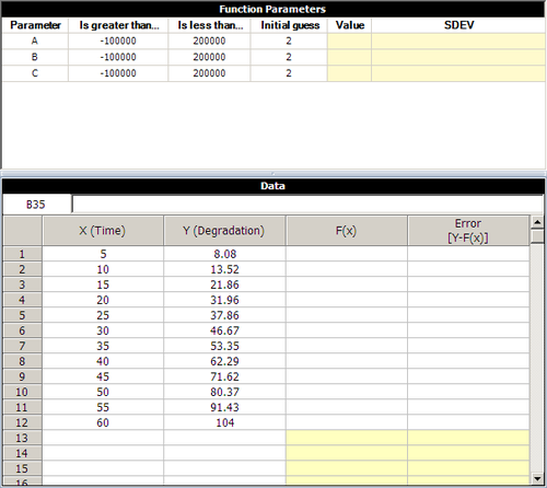
Step 1: Insert an Equation Fit Solver folio in your project and enter the given data in the folio, as shown next.
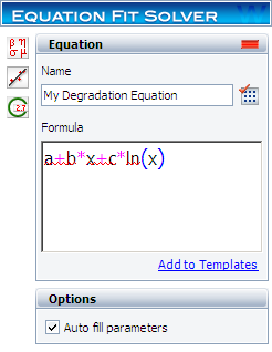
Step 2: Enter the degradation equation in the control panel and name it “My Degradation Equation,” as shown next.
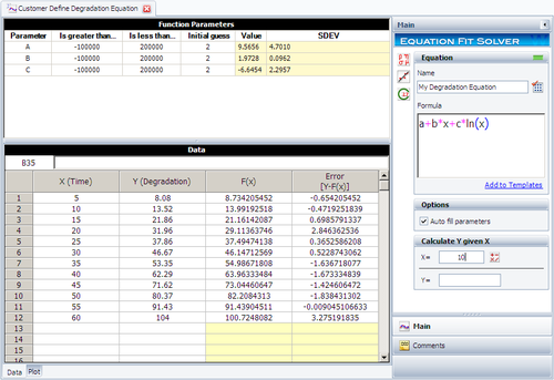
Step 3: Click Calculate. The following picture shows the results.
Step 4: You can use the Calculate Y given X area on the control panel to make predictions. For example, the predicted Y value at X=100 is 176.2424.
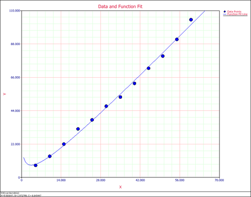
Step 5: The following plot shows the fitted model and the observed values.


