The Generalized Gamma Distribution: Difference between revisions
| Line 72: | Line 72: | ||
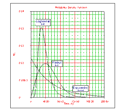
As mentioned previously, the generalized gamma distribution includes other distributions as special cases based on the values of the parameters. | As mentioned previously, the generalized gamma distribution includes other distributions as special cases based on the values of the parameters. | ||
[[Image:ldagamma10.1.gif|thumb|center| | [[Image:ldagamma10.1.gif|thumb|center|400px| ]] | ||
• The Weibull distribution is a special case when <math>\lambda =1</math> and: | • The Weibull distribution is a special case when <math>\lambda =1</math> and: | ||
Revision as of 17:13, 15 August 2011
The Generalized Gamma Distribution
While not as frequently used for modeling life data as the previous distributions, the generalized gamma distribution does have the ability to mimic the attributes of other distributions such as the Weibull or lognormal, based on the values of the distribution's parameters. While the generalized gamma distribution is not often used to model life data by itself , its ability to behave like other more commonly-used life distributions is sometimes used to determine which of those life distributions should be used to model a particular set of data.
Generalized Gamma Probability Density Function
The generalized gamma function is a three-parameter distribution. One version of the generalized gamma distribution uses the parameters [math]\displaystyle{ k }[/math], [math]\displaystyle{ \beta }[/math], and [math]\displaystyle{ \theta }[/math]. The [math]\displaystyle{ pdf }[/math] for this form of the generalized gamma distribution is given by:
- [math]\displaystyle{ f(t)=\frac{\beta }{\Gamma (k)\cdot \theta }{{\left( \frac{t}{\theta } \right)}^{k\beta -1}}{{e}^{-{{\left( \tfrac{t}{\theta } \right)}^{\beta }}}} }[/math]
where [math]\displaystyle{ \theta \gt 0 }[/math] is a scale parameter, [math]\displaystyle{ \beta \gt 0 }[/math] and [math]\displaystyle{ k\gt 0 }[/math] are shape parameters and [math]\displaystyle{ \Gamma (x) }[/math] is the gamma function of [math]\displaystyle{ x }[/math], which is defined by:
- [math]\displaystyle{ \Gamma (x)=\int_{0}^{\infty }{{s}^{x-1}}\cdot {{e}^{-s}}ds }[/math]
With this version of the distribution, however, convergence problems arise that severely limit its usefulness. Even with data sets containing 200 or more data points, the MLE methods may fail to converge. Further adding to the confusion is the fact that distributions with widely different values of [math]\displaystyle{ k }[/math], [math]\displaystyle{ \beta }[/math], and [math]\displaystyle{ \theta }[/math] may appear almost identical [21]. In order to overcome these difficulties, Weibull++ uses a reparameterization with parameters [math]\displaystyle{ \mu }[/math] , [math]\displaystyle{ \sigma }[/math] , and [math]\displaystyle{ \lambda }[/math] [21] where:
- [math]\displaystyle{ \begin{align} \mu = & ln(\theta )+\frac{1}{\beta }\cdot ln\left( \frac{1}{{{\lambda }^{2}}} \right) \\ \sigma = & \frac{1}{\beta \sqrt{k}} \\ \lambda = & \frac{1}{\sqrt{k}} \end{align} }[/math]
where [math]\displaystyle{ -\infty \lt \mu \lt \infty ,\,\sigma \gt 0, }[/math] and [math]\displaystyle{ 0\lt \lambda . }[/math] While this makes the distribution converge much more easily in computations, it does not facilitate manual manipulation of the equation. By allowing [math]\displaystyle{ \lambda }[/math] to become negative, the [math]\displaystyle{ pdf }[/math] of the reparameterized distribution is given by:
- [math]\displaystyle{ f(t)=\left\{ \begin{matrix} \tfrac{|\lambda |}{\sigma \cdot t}\cdot \tfrac{1}{\Gamma \left( \tfrac{1}{{{\lambda }^{2}}} \right)}\cdot {{e}^{\left[ \tfrac{\lambda \cdot \tfrac{\text{ln}(t)-\mu }{\sigma }+\text{ln}\left( \tfrac{1}{{{\lambda }^{2}}} \right)-{{e}^{\lambda \cdot \tfrac{\text{ln}(t)-\mu }{\sigma }}}}{{{\lambda }^{2}}} \right]}}\text{ if }\lambda \ne 0 \\ \tfrac{1}{t\cdot \sigma \sqrt{2\pi }}{{e}^{-\tfrac{1}{2}{{\left( \tfrac{\text{ln}(t)-\mu }{\sigma } \right)}^{2}}}}\text{ if }\lambda =0 \\ \end{matrix} \right. }[/math]
Generalized Gamma Reliability Function
The reliability function for the generalized gamma distribution is given by:
- [math]\displaystyle{ R(t)=\left\{ \begin{array}{*{35}{l}} 1-{{\Gamma }_{I}}\left( \tfrac{{{e}^{\lambda \left( \tfrac{\text{ln}(t)-\mu }{\sigma } \right)}}}{{{\lambda }^{2}}};\tfrac{1}{{{\lambda }^{2}}} \right)\text{ if }\lambda \gt 0 \\ 1-\Phi \left( \tfrac{\text{ln}(t)-\mu }{\sigma } \right)\text{ if }\lambda =0 \\ {{\Gamma }_{I}}\left( \tfrac{{{e}^{\lambda \left( \tfrac{\text{ln}(t)-\mu }{\sigma } \right)}}}{{{\lambda }^{2}}};\tfrac{1}{{{\lambda }^{2}}} \right)\text{ if }\lambda \lt 0 \\ \end{array} \right. }[/math]
where:
- [math]\displaystyle{ \Phi (z)=\frac{1}{\sqrt{2\pi }}\int_{-\infty }^{z}{{e}^{-\tfrac{{{x}^{2}}}{2}}}dx }[/math]
and [math]\displaystyle{ {{\Gamma }_{I}}(k;x) }[/math] is the incomplete gamma function of [math]\displaystyle{ k }[/math]
and [math]\displaystyle{ x }[/math] , which is given by:
- [math]\displaystyle{ {{\Gamma }_{I}}(k;x)=\frac{1}{\Gamma (k)}\int_{0}^{x}{{s}^{k-1}}{{e}^{-s}}ds }[/math]
where [math]\displaystyle{ \Gamma (x) }[/math] is the gamma function of [math]\displaystyle{ x }[/math] . Note that in Weibull++ the probability plot of the generalized gamma is created on lognormal probability paper. This means that the fitted line will not be straight unless [math]\displaystyle{ \lambda =0. }[/math]
Generalized Gamma Failure Rate Function
As defined in Chapter 3, the failure rate function is given by:
- [math]\displaystyle{ \lambda (t)=\frac{f(t)}{R(t)} }[/math]
Owing to the complexity of the equations involved, the function will not be displayed here, but the failure rate function for the generalized gamma distribution can be obtained merely by dividing Eqn. (ggampdf) by Eqn. (ggamrel).
Generalized Gamma Reliable Life
The reliable life, [math]\displaystyle{ {{T}_{R}} }[/math] , of a unit for a specified reliability, starting the mission at age zero, is given by:
[math]\displaystyle{ {{T}_{R}}=\left\{ \begin{array}{*{35}{l}} {{e}^{\mu +\tfrac{\sigma }{\lambda }\ln \left[ {{\lambda }^{2}}\Gamma _{I}^{-1}\left( 1-R,\tfrac{1}{{{\lambda }^{2}}} \right) \right]}}\text{ if }\lambda \gt 0 \\ {{\Phi }^{-1}}(1-R)\text{ if }\lambda =0 \\ {{e}^{\mu +\tfrac{\sigma }{\lambda }\ln \left[ {{\lambda }^{2}}\Gamma _{I}^{-1}\left( R,\tfrac{1}{{{\lambda }^{2}}} \right) \right]}}\text{ if }\lambda \lt 0 \\ \end{array} \right. }[/math]
Characteristics of the Generalized Gamma Distribution
As mentioned previously, the generalized gamma distribution includes other distributions as special cases based on the values of the parameters.
• The Weibull distribution is a special case when [math]\displaystyle{ \lambda =1 }[/math] and:
- [math]\displaystyle{ \begin{align} & \beta = & \frac{1}{\sigma } \\ & \eta = & \ln (\mu ) \end{align} }[/math]
• In this case, the generalized distribution has the same behavior as the Weibull for [math]\displaystyle{ \sigma \gt 1, }[/math] [math]\displaystyle{ \sigma =1, }[/math] and [math]\displaystyle{ \sigma \lt 1 }[/math] ( [math]\displaystyle{ \beta \lt 1, }[/math] [math]\displaystyle{ \beta =1, }[/math] and [math]\displaystyle{ \beta \gt 1 }[/math] respectively).
• The exponential distribution is a special case when [math]\displaystyle{ \lambda =1 }[/math] and [math]\displaystyle{ \sigma =1 }[/math].
• The lognormal distribution is a special case when [math]\displaystyle{ \lambda =0 }[/math].
• The gamma distribution is a special case when [math]\displaystyle{ \lambda =\sigma }[/math].
By allowing [math]\displaystyle{ \lambda }[/math] to take negative values, the generalized gamma distribution can be further extended to include additional distributions as special cases. For example, the Fréchet distribution of maxima (also known as a reciprocal Weibull) is a special case when [math]\displaystyle{ \lambda =-1 }[/math].
Confidence Bounds
The only method available in Weibull++ for confidence bounds for the generalized gamma distribution is the Fisher matrix, which is described next.
Bounds on the Parameters
The lower and upper bounds on the parameter [math]\displaystyle{ \mu }[/math] are estimated from:
- [math]\displaystyle{ \begin{align} & {{\mu }_{U}}= & \widehat{\mu }+{{K}_{\alpha }}\sqrt{Var(\widehat{\mu })}\text{ (upper bound)} \\ & {{\mu }_{L}}= & \widehat{\mu }-{{K}_{\alpha }}\sqrt{Var(\widehat{\mu })}\text{ (lower bound)} \end{align} }[/math]
For the parameter [math]\displaystyle{ \widehat{\sigma } }[/math] , [math]\displaystyle{ \ln (\widehat{\sigma }) }[/math] is treated as normally distributed, and the bounds are estimated from:
- [math]\displaystyle{ \begin{align} & {{\sigma }_{U}}= & \widehat{\sigma }\cdot {{e}^{\tfrac{{{K}_{\alpha }}\sqrt{Var(\widehat{\sigma })}}{\widehat{\sigma }}}}\text{ (upper bound)} \\ & {{\sigma }_{L}}= & \frac{\widehat{\sigma }}{{{e}^{\tfrac{{{K}_{\alpha }}\sqrt{Var(\widehat{\sigma })}}{\widehat{\sigma }}}}}\text{ (lower bound)} \end{align} }[/math]
For the parameter [math]\displaystyle{ \lambda , }[/math] the bounds are estimated from:
- [math]\displaystyle{ \begin{align} & {{\lambda }_{U}}= & \widehat{\lambda }+{{K}_{\alpha }}\sqrt{Var(\widehat{\lambda })}\text{ (upper bound)} \\ & {{\lambda }_{L}}= & \widehat{\lambda }-{{K}_{\alpha }}\sqrt{Var(\widehat{\lambda })}\text{ (lower bound)} \end{align} }[/math]
where [math]\displaystyle{ {{K}_{\alpha }} }[/math] is defined by:
- [math]\displaystyle{ \alpha =\frac{1}{\sqrt{2\pi }}\int_{{{K}_{\alpha }}}^{\infty }{{e}^{-\tfrac{{{t}^{2}}}{2}}}dt=1-\Phi ({{K}_{\alpha }}) }[/math]
If [math]\displaystyle{ \delta }[/math] is the confidence level, then [math]\displaystyle{ \alpha =\tfrac{1-\delta }{2} }[/math] for the two-sided bounds, and [math]\displaystyle{ \alpha =1-\delta }[/math] for the one-sided bounds.
The variances and covariances of [math]\displaystyle{ \widehat{\mu } }[/math] and [math]\displaystyle{ \widehat{\sigma } }[/math] are estimated as follows:
- [math]\displaystyle{ \begin{align} & & \left( \begin{matrix} \widehat{Var}\left( \widehat{\mu } \right) & \widehat{Cov}\left( \widehat{\mu },\widehat{\sigma } \right) & \widehat{Cov}\left( \widehat{\mu },\widehat{\lambda } \right) \\ \widehat{Cov}\left( \widehat{\sigma },\widehat{\mu } \right) & \widehat{Var}\left( \widehat{\sigma } \right) & \widehat{Cov}\left( \widehat{\sigma },\widehat{\lambda } \right) \\ \widehat{Cov}\left( \widehat{\lambda },\widehat{\mu } \right) & \widehat{Cov}\left( \widehat{\lambda },\widehat{\sigma } \right) & \widehat{Var}\left( \widehat{\lambda } \right) \\ \end{matrix} \right) \\ & = & \left( \begin{matrix} -\tfrac{{{\partial }^{2}}\Lambda }{\partial {{\mu }^{2}}} & -\tfrac{{{\partial }^{2}}\Lambda }{\partial \mu \partial \sigma } & -\tfrac{{{\partial }^{2}}\Lambda }{\partial \mu \partial \lambda } \\ -\tfrac{{{\partial }^{2}}\Lambda }{\partial \mu \partial \sigma } & -\tfrac{{{\partial }^{2}}\Lambda }{\partial {{\sigma }^{2}}} & -\tfrac{{{\partial }^{2}}\Lambda }{\partial \lambda \partial \sigma } \\ -\tfrac{{{\partial }^{2}}\Lambda }{\partial \mu \partial \lambda } & -\tfrac{{{\partial }^{2}}\Lambda }{\partial \lambda \partial \sigma } & -\tfrac{{{\partial }^{2}}\Lambda }{\partial {{\lambda }^{2}}} \\ \end{matrix} \right)_{\mu =\widehat{\mu },\sigma =\widehat{\sigma },\lambda =\hat{\lambda }}^{-1} \end{align} }[/math]
Where [math]\displaystyle{ \Lambda }[/math] is the log-likelihood function of the generalized gamma distribution.
Bounds on Reliability
The upper and lower bounds on reliability are given by:
- [math]\displaystyle{ \begin{align} & {{R}_{U}}= & \frac{{\hat{R}}}{\hat{R}+(1-\hat{R}){{e}^{-\tfrac{{{K}_{\alpha }}\sqrt{Var(\widehat{R})}}{\hat{R}(1-\hat{R})}}}} \\ & {{R}_{L}}= & \frac{{\hat{R}}}{\hat{R}+(1-\hat{R}){{e}^{\tfrac{{{K}_{\alpha }}\sqrt{Var(\widehat{R})}}{\hat{R}(1-\hat{R})}}}} \end{align} }[/math]
where:
- [math]\displaystyle{ \begin{align} & Var(\widehat{R})= & {{\left( \frac{\partial R}{\partial \mu } \right)}^{2}}Var(\widehat{\mu })+{{\left( \frac{\partial R}{\partial \sigma } \right)}^{2}}Var(\widehat{\sigma })+{{\left( \frac{\partial R}{\partial \lambda } \right)}^{2}}Var(\widehat{\lambda })+ \\ & & +2\left( \frac{\partial R}{\partial \mu } \right)\left( \frac{\partial R}{\partial \sigma } \right)Cov(\widehat{\mu },\widehat{\sigma })+2\left( \frac{\partial R}{\partial \mu } \right)\left( \frac{\partial R}{\partial \lambda } \right)Cov(\widehat{\mu },\widehat{\lambda })+ \\ & & +2\left( \frac{\partial R}{\partial \lambda } \right)\left( \frac{\partial R}{\partial \sigma } \right)Cov(\widehat{\lambda },\widehat{\sigma }) \end{align} }[/math]
Bounds on Time
The bounds around time for a given percentile, or unreliability, are estimated by first solving the reliability equation with respect to time, given by Eqn. (GGamma Time). Since [math]\displaystyle{ T }[/math] is a positive variable, the transformed variable [math]\displaystyle{ \hat{u}=\ln (\widehat{T}) }[/math] is treated as normally distributed and the bounds are estimated from:
- [math]\displaystyle{ \begin{align} & {{u}_{u}}= & \ln {{T}_{U}}=\widehat{u}+{{K}_{\alpha }}\sqrt{Var(\widehat{u})} \\ & {{u}_{L}}= & \ln {{T}_{L}}=\widehat{u}-{{K}_{\alpha }}\sqrt{Var(\widehat{u})} \end{align} }[/math]
Solving for [math]\displaystyle{ {{T}_{U}} }[/math] and [math]\displaystyle{ {{T}_{L}} }[/math] we get:
- [math]\displaystyle{ \begin{align} & {{T}_{U}}= & {{e}^{{{T}_{U}}}}\text{ (upper bound)} \\ & {{T}_{L}}= & {{e}^{{{T}_{L}}}}\text{ (lower bound)} \end{align} }[/math]
The variance of [math]\displaystyle{ u }[/math] is estimated from:
- [math]\displaystyle{ \begin{align} & Var(\widehat{u})= & {{\left( \frac{\partial u}{\partial \mu } \right)}^{2}}Var(\widehat{\mu })+{{\left( \frac{\partial u}{\partial \sigma } \right)}^{2}}Var(\widehat{\sigma })+{{\left( \frac{\partial u}{\partial \lambda } \right)}^{2}}Var(\widehat{\lambda })+ \\ & & +2\left( \frac{\partial u}{\partial \mu } \right)\left( \frac{\partial u}{\partial \sigma } \right)Cov(\widehat{\mu },\widehat{\sigma })+2\left( \frac{\partial u}{\partial \mu } \right)\left( \frac{\partial u}{\partial \lambda } \right)Cov(\widehat{\mu },\widehat{\lambda })+ \\ & & +2\left( \frac{\partial u}{\partial \lambda } \right)\left( \frac{\partial u}{\partial \sigma } \right)Cov(\widehat{\lambda },\widehat{\sigma }) \end{align} }[/math]
A Generalized Gamma Distribution Example
The following data set represents revolutions-to-failure (in millions) for 23 ball bearings in a fatigue test [21].
- [math]\displaystyle{ \begin{array}{*{35}{l}} \text{17}\text{.88} & \text{28}\text{.92} & \text{33} & \text{41}\text{.52} & \text{42}\text{.12} & \text{45}\text{.6} & \text{48}\text{.4} & \text{51}\text{.84} & \text{51}\text{.96} & \text{54}\text{.12} \\ \text{55}\text{.56} & \text{67}\text{.8} & \text{68}\text{.64} & \text{68}\text{.64} & \text{68}\text{.88} & \text{84}\text{.12} & \text{93}\text{.12} & \text{98}\text{.64} & \text{105}\text{.12} & \text{105}\text{.84} \\ \text{127}\text{.92} & \text{128}\text{.04} & \text{173}\text{.4} & {} & {} & {} & {} & {} & {} & {} \\ \end{array} }[/math]
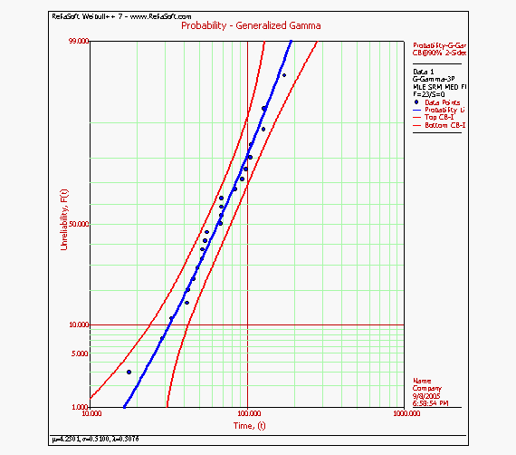
When the generalized gamma distribution is fitted to this data using MLE, the following values for parameters are obtained:
- [math]\displaystyle{ \begin{align} & \widehat{\mu }= & 4.23064 \\ & \widehat{\sigma }= & 0.509982 \\ & \widehat{\lambda }= & 0.307639 \end{align} }[/math]
Note that for this data, the generalized gamma offers a compromise between the Weibull [math]\displaystyle{ (\lambda =1), }[/math] and the lognormal [math]\displaystyle{ (\lambda =0) }[/math] distributions. The value of [math]\displaystyle{ \lambda }[/math] indicates that the lognormal distribution is better supported by the data. A better assessment, however, can be made by looking at the confidence bounds on [math]\displaystyle{ \lambda . }[/math] For example, the 90% two-sided confidence bounds are:
- [math]\displaystyle{ \begin{align} & {{\lambda }_{u}}= & -0.592087 \\ & {{\lambda }_{u}}= & 1.20736 \end{align} }[/math]
It can be then concluded that both distributions (i.e. Weibull and lognormal) are well supported by the data, with the lognormal being the ,better supported of the two. In Weibull++ the generalized gamma probability is plotted on gamma probability paper, as shown next.
It is important to also note that as in the case of the mixed Weibull distribution, in the case of regression analysis, using a generalized gamma model, the choice of regression axis, i.e. [math]\displaystyle{ RRX }[/math] or [math]\displaystyle{ RRY, }[/math] is of no consequence since non-linear regression is utilized.


