Template:Lognormal distribution probability plotting
Probability Plotting
As described before, probability plotting involves plotting the failure times and associated unreliability estimates on specially constructed probability plotting paper. The form of this paper is based on a linearization of the [math]\displaystyle{ cdf }[/math] of the specific distribution. For the lognormal distribution, the cumulative density function can be written as:
- [math]\displaystyle{ F({T}')=\Phi \left( \frac{{T}'-{\mu }'}{{{\sigma }_{{{T}'}}}} \right) }[/math]
- or:
- [math]\displaystyle{ {{\Phi }^{-1}}\left[ F({T}') \right]=-\frac{{{\mu }'}}{{{\sigma }_{{{T}'}}}}+\frac{1}{{{\sigma }_{{{T}'}}}}\cdot {T}' }[/math]
- where:
- [math]\displaystyle{ \Phi (x)=\frac{1}{\sqrt{2\pi }}\int_{-\infty }^{x}{{e}^{-\tfrac{{{t}^{2}}}{2}}}dx }[/math]
- Now, let:
- [math]\displaystyle{ y={{\Phi }^{-1}}\left[ F({T}') \right] }[/math]
- [math]\displaystyle{ a=-\frac{{{\mu }'}}{{{\sigma }_{{{T}'}}}} }[/math]
- and:
- [math]\displaystyle{ b=\frac{1}{{{\sigma }_{{{T}'}}}} }[/math]
which results in the linear equation of:
- [math]\displaystyle{ y=a+b{T}' }[/math]
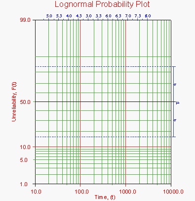
The normal probability paper resulting from this linearized [math]\displaystyle{ cdf }[/math] function is shown next.
The process for reading the parameter estimate values from the lognormal probability plot is very similar to the method employed for the normal distribution (see Chapter 8). However, since the lognormal distribution models the natural logarithms of the times-to-failure, the values of the parameter estimates must be read and calculated based on a logarithmic scale, as opposed to the linear time scale as it was done with the normal distribution. This parameter scale appears at the top of the lognormal probability plot.
The process of lognormal probability plotting is illustrated in the following example.
Example 1
Eight units are put on a life test and tested to failure. The failures occurred at 45, 140, 260, 500, 850, 1400, 3000, and 9000 hours. Estimate the parameters for the lognormal distribution using probability plotting.
Solution to Example 1
In order to plot the points for the probability plot, the appropriate unreliability estimate values must be obtained. These will be estimated through the use of median ranks, which can be obtained from statistical tables or the Quick Statistical Reference in Weibull++. The following table shows the times-to-failure and the appropriate median rank values for this example:
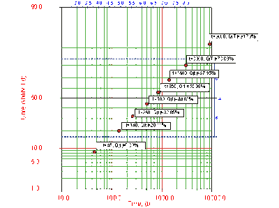
These points may now be plotted on normal probability plotting paper as shown in the next figure.
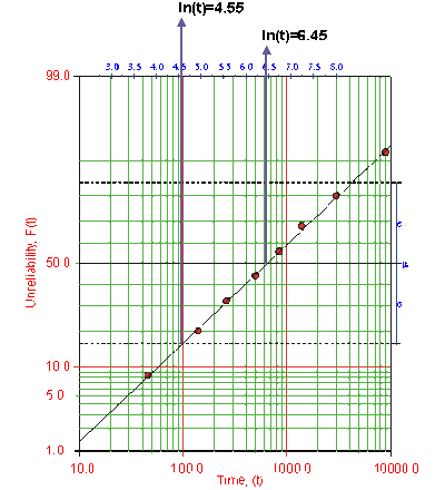
Draw the best possible line through the plot points. The time values where this line intersects the 15.85% and 50% unreliability values should be projected up to the logarithmic scale, as shown in the following plot.
The natural logarithm of the time where the fitted line intersects .. is equivalent to [math]\displaystyle{ {\mu }' }[/math] . In this case, [math]\displaystyle{ {\mu }'=6.45 }[/math] . The value for [math]\displaystyle{ {{\sigma }_{{{T}'}}} }[/math] is equal to the difference between the natural logarithms of the times where the fitted line crosses [math]\displaystyle{ Q(t)=50% }[/math] and [math]\displaystyle{ Q(t)=15.85%. }[/math] At [math]\displaystyle{ Q(t)=15.85% }[/math] , ln [math]\displaystyle{ (t)=4.55 }[/math] . Therefore, [math]\displaystyle{ {{\sigma }_{{{T}'}}}=6.45-4.55=1.9 }[/math] .


