Template:Failure modes configurations
Failure Modes Configurations
Series Configuration
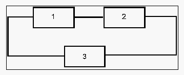
The basic competing failure modes configuration, which has already been discussed, is a series configuration. In a series configuration, the occurrence of any failure mode results in failure for the product.
The equation that describes series configuration is:
- [math]\displaystyle{ R(t)={{R}_{1}}(t)\cdot {{R}_{2}}(t)\cdot ...\cdot {{R}_{n}}(t) }[/math]
where [math]\displaystyle{ n }[/math] is the total number of failure modes considered.
Parallel
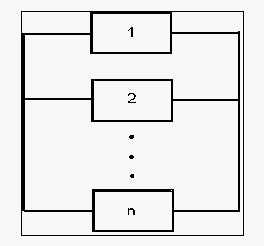
In a simple parallel configuration, at least one of the failure modes must not occur for the product to continue operation.
[math]\displaystyle{ }[/math]
The equation that describes parallel configuration is:
- [math]\displaystyle{ R(t)=1-\underset{i=1}{\overset{n}{\mathop \prod }}\,(1-{{R}_{i}}(t)) }[/math]
where [math]\displaystyle{ n }[/math] is the total number of failure modes considered.
Combination of Series and Parallel
While many smaller products can be accurately represented by either a simple series or parallel configuration, there may be larger products that involve both series and parallel configurations in the overall model of the product. Such products can be analyzed by calculating the reliabilities for the individual series and parallel sections and then combining them in the appropriate manner.
[math]\displaystyle{ }[/math]
k-out-of-n Parallel Configuration
The k-out-of-n configuration is a special case of parallel redundancy. This type of configuration requires that at least [math]\displaystyle{ k }[/math] failure modes do not happen out of the total [math]\displaystyle{ n }[/math] parallel failure modes for the product to succeed. The simplest case of a k-out-of-n configuration is when the failure modes are independent and identical and have the same failure distribution and uncertainties about the parameters (in other words they are derived from the same test data). In this case, the reliability of the product with such a configuration can be evaluated using the binomial distribution, or:
- [math]\displaystyle{ R(t)=\overset{n}{\mathop{\underset{r=k}{\mathop{\underset{}{\overset{}{\mathop \sum }}\,}}\,}}\,\left( \underset{k}{\mathop{\overset{n}{\mathop{{}}}\,}}\, \right){{R}^{r}}(t){{(1-R(t))}^{n-r}} }[/math]
In the case where the k-out-of-n failure modes are not identical, other approaches for calculating the reliability must be used (e.g. the event space method). Discussion of these is beyond the scope of this reference. Interested readers can consult ReliaSoft's System Reliability Reference.
Complex Systems
In many cases, it is not easy to recognize which components are in series and which are in parallel in a complex system.
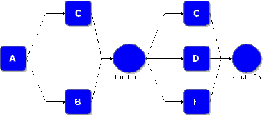
The previous configuration cannot be broken down into a group of series and parallel configurations. This is primarily due to the fact that failure mode C has two paths leading away from it, whereas B and D have only one. Several methods exist for obtaining the reliability of a complex configuration including the decomposition method, the event space method and the path-tracing method. Discussion of these is beyond the scope of this reference. Interested readers can consult ReliaSoft's System Reliability Reference.
Example 14
Assume that a product has five failure modes: A, B, C, D and F. Furthermore, assume that failure of the product will occur if mode A occurs, modes B and C occur simultaneously or if either modes C and D, C and F or D and F occur simultaneously. Times-to-failure for each mode is given in the next table.
The RBD that describes this configuration is shown next.
[math]\displaystyle{ }[/math]
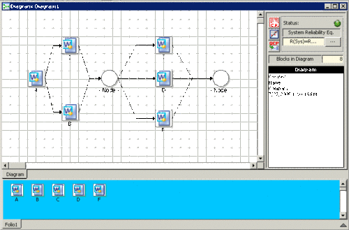
One folio with multiple data sheets was created in Weibull++ for each of the data sets and each file was analyzed using the two-parameter Weibull distribution, MLE as the analysis method and Fisher Matrix as the confidence bounds method. A diagram is created by choosing Add Diagram from the Project menu. The failure modes can be inserted into the diagram by dragging them from the template. The nodes are inserted by clicking choosing Add Node from the Diagram menu.
[math]\displaystyle{ }[/math]
The number of required paths can be specified by double clicking the node and entering the appropriate number (1 in the first node and 2 in the second node).
[math]\displaystyle{ }[/math]
Using the Quick Calculation Pad (QCP), the estimated R( [math]\displaystyle{ 100 }[/math] hours [math]\displaystyle{ ) }[/math] and the 90% two-sided confidence bounds are:
- [math]\displaystyle{ \begin{matrix} {{{\hat{R}}}_{U}}(100)=0.991 \\ \hat{R}(100)=0.9905 \\ {{{\hat{R}}}_{L}}(100)=0.9080 \\ \end{matrix} }[/math]


