Linearity and Bias Study Example
New format available! This reference is now available in a new format that offers faster page load, improved display for calculations and images and more targeted search.
As of January 2024, this Reliawiki page will not continue to be updated. Please update all links and bookmarks to the latest references at DOE examples and DOE reference examples.
This example appears in the Experiment Design and Analysis Reference book.
If a baby is 8.5 lbs and the reading of a scale is 8.9 lbs, then the bias is 0.4 lb. If an adult is 85 lbs and the reading from the same scale is 85.4 lbs, then the bias is still 0.4 lb. This scale does not seem to have a linearity issue. However, if the reading for the adult were 89 lbs, the bias would seem to increase as the weight increases. Thus, you might suspect that the scale has a linearity issue.
The following data set shows measurements from a gage linearity and bias study.
| Part | Reference | Reading | Part | Reference | Reading |
|---|---|---|---|---|---|
| 1 | 2 | 1.95 | 3 | 6 | 6.04 |
| 1 | 2 | 2.10 | 3 | 6 | 6.25 |
| 1 | 2 | 2.00 | 3 | 6 | 6.21 |
| 1 | 2 | 1.92 | 3 | 6 | 6.16 |
| 1 | 2 | 1.97 | 3 | 6 | 6.06 |
| 1 | 2 | 1.94 | 3 | 6 | 6.03 |
| 1 | 2 | 2.02 | 4 | 8 | 8.40 |
| 1 | 2 | 2.05 | 4 | 8 | 8.35 |
| 1 | 2 | 1.95 | 4 | 8 | 8.15 |
| 1 | 2 | 2.04 | 4 | 8 | 8.10 |
| 2 | 4 | 4.09 | 4 | 8 | 8.18 |
| 2 | 4 | 4.16 | 5 | 10 | 10.49 |
| 2 | 4 | 4.16 | 5 | 10 | 10.28 |
| 2 | 4 | 4.10 | 5 | 10 | 10.42 |
| 2 | 4 | 4.06 | 5 | 10 | 10.29 |
| 2 | 4 | 4.11 | 5 | 10 | 10.14 |
| 2 | 4 | 4.02 | 5 | 10 | 10.07 |
The first column is the part ID. The second column is the “true” value of each part, called reference or master. In a linearity study, the selected reference should cover the minimal and maximal value of the produced parts. The Reading column is the observed value from a measurement device. Each part was measured multiple times, and some parts have the same reference value.
The following linear regression equation is used for gage linearity and bias study:
- [math]\displaystyle{ Y={{\beta }_{0}}+{{\beta }_{1}}X+\varepsilon }[/math]
where:
- Y is the bias.
- X is the reference value.
- [math]\displaystyle{ {{\beta }_{0}} }[/math] and [math]\displaystyle{ {{\beta }_{1}} }[/math] are the coefficients.
- [math]\displaystyle{ \varepsilon }[/math] is error following a normal distribution
- [math]\displaystyle{ N\left( 0,{{\sigma }^{2}} \right) }[/math]
First, we need to calculate the bias for each observation in the above table. Bias is the difference between “Reading and Reference. The bias values are:
Part Reference Reading Bias Part Reference Reading Bias 1 2 1.95 -0.05 3 6 6.04 0.04 1 2 2.1 0.1 3 6 6.25 0.25 1 2 2 0 3 6 6.21 0.21 1 2 1.92 -0.08 3 6 6.16 0.16 1 2 1.97 -0.03 3 6 6.06 0.06 1 2 1.94 -0.06 3 6 6.03 0.03 1 2 2.02 0.02 4 8 8.4 0.4 1 2 2.05 0.05 4 8 8.35 0.35 1 2 1.95 -0.05 4 8 8.15 0.15 1 2 2.04 0.04 4 8 8.1 0.1 2 4 4.09 0.09 4 8 8.18 0.18 2 4 4.16 0.16 5 10 10.49 0.49 2 4 4.16 0.16 5 10 10.28 0.28 2 4 4.1 0.1 5 10 10.42 0.42 2 4 4.06 0.06 5 10 10.29 0.29 2 4 4.11 0.11 5 10 10.14 0.14 2 4 4.02 0.02 5 10 10.07 0.07
Results for Linearity Study
Using the Reference column as X and the Bias column as Y in the linear regression, we get the following results:
Source of Variation Degrees of Freedom Sum of Squares [Partial] Mean Squares [Partial] F Ratio P Value Reference 1 0.3748 0.3748 40.4619 3.83E-07 Residual 32 0.2964 0.0093 Lack of Fit 3 0.01 0.0033 0.3388 0.7974 Pure Error 29 0.2864 0.0099 Total 33 0.6712
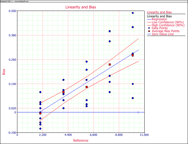
The calculated R-sq is 55.84% and R-sq(adj) is 54.46%. These values are not very high due to the large variation among the bias values. However, the p value of the lack of fit shows that the linear equation fits the data very well, and the following plot also shows there is a linear relation between reference and bias.
The estimated coefficients are:
Regression Information Term Coefficient Standard Error Low CI High CI T Value P Value Intercept -0.0685 0.0347 -0.1272 -0.0098 -1.9773 0.0567 Reference 0.0358 0.0056 0.0263 0.0454 6.361 3.83E-07
The linearity is defined by:
- [math]\displaystyle{ \begin{align} & \text{linearity}=|{{\beta }_{1}}|\times \text{process variation} \\ & \text{= }\!\!|\!\!\text{ }{{\beta }_{1}}|\times 6\times \text{process standard deviation} \end{align} }[/math]
This means that when this gage is used for a process, the observed process variation will be [math]\displaystyle{ |{{\beta }_{1}}| }[/math] times larger than the true process variation. This is because the observed value of a part is [math]\displaystyle{ |{{\beta }_{1}}| }[/math] times larger/smaller than the true value plus a constant value of the intercept.
The percentage of linearity (% linearity) is defined by:
- [math]\displaystyle{ \text{ }\!\!%\!\!\text{ linearity}=100\left( \frac{\text{linearity}}{\text{process variation}} \right)%=\left( 100{{\beta }_{1}} \right)% }[/math]
% linearity shows the percentage of increase of the process variation due to the linearity of the gage. The smaller the linearity, the better the gage is.
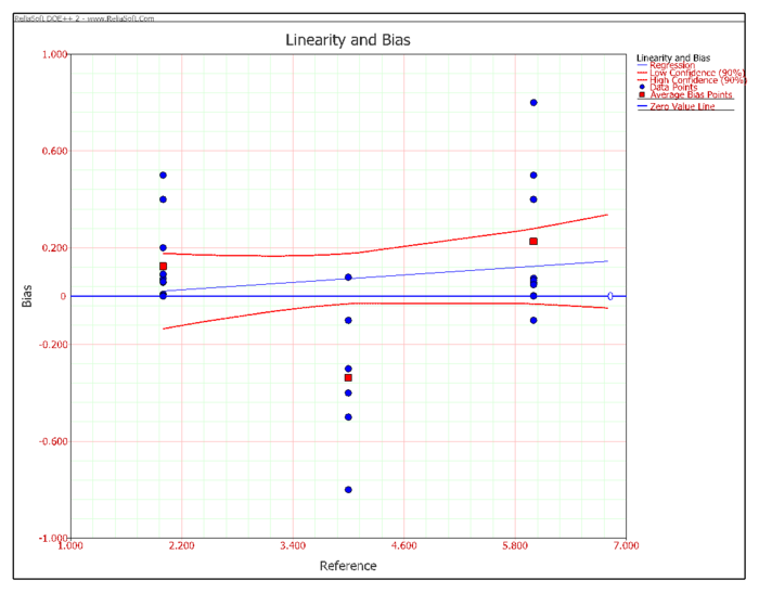
If the linearity study shows no linear relation between reference and bias, you need to check the scatter plot of reference and bias to see if there is a non-linear relation. For example, the following plot shows a non-linear relationship between reference and bias.
Although the slope in the linear equation is almost 0 in the above plot, it does not mean the gage is accurate. The above figure shows an obvious V-shaped pattern between reference and bias. This non-linear pattern requires further analysis to judge whether the gage’s accuracy is acceptable.
Results for Bias Study
The bias study results are:
Reference Bias %Bias Std of Mean t p Average 0.1253 2.09% 0.017 7.3517 0.0000 2 -0.0060 0.10% 0.0183 0.3284 0.7501 4 0.1000 1.67% 0.0191 5.2223 0.0020 6 0.1250 2.08% 0.0385 3.2437 0.0229 8 0.2360 3.93% 0.0587 4.0203 0.0159 10 0.2817 4.70% 0.0652 4.3209 0.0076
- The Average row is the average of all the bias values while other rows are the reference values used in the study.
- The second column is the average bias for each reference value.
- The 3rd column is [math]\displaystyle{ |bias|/\text{process variation}\times \text{100 }\!\!%\!\!\text{ } }[/math]. Process variation is commonly defined as 6 times the process standard deviation. For this example, the process standard deviation is set to 1 and the process variation is 6.
- The 4th column is the standard deviation of the mean value of the bias for each reference value. If there are multiple parts having the same reference value, it is the pooled standard deviation of all the parts.
The T value is the ratio of the absolute value of the 2nd column and the 4th column. The p value is calculated from the T value and the corresponding degree of freedom for each reference value. If the p value is smaller than a given significance level, say 0.05, then the corresponding row has significant bias.
For this example, the p value column shows that bias appears for all the reference values except for the reference value of 2. The p value for Average row is very small, which means the average bias of all the readings is significant.
In some cases, such as the figure in the previous section, non-linearity occurs. Bias values are negative for some of the references and positive for others. Although each of the reference values can have significant bias, the average bias of all the references may not be significant.
When there are multiple parts for the same reference value, the standard deviation for that reference value is the pooled standard deviation of all the parts with the same reference value. The standard deviation for the average is calculated from the variance of all the parts.
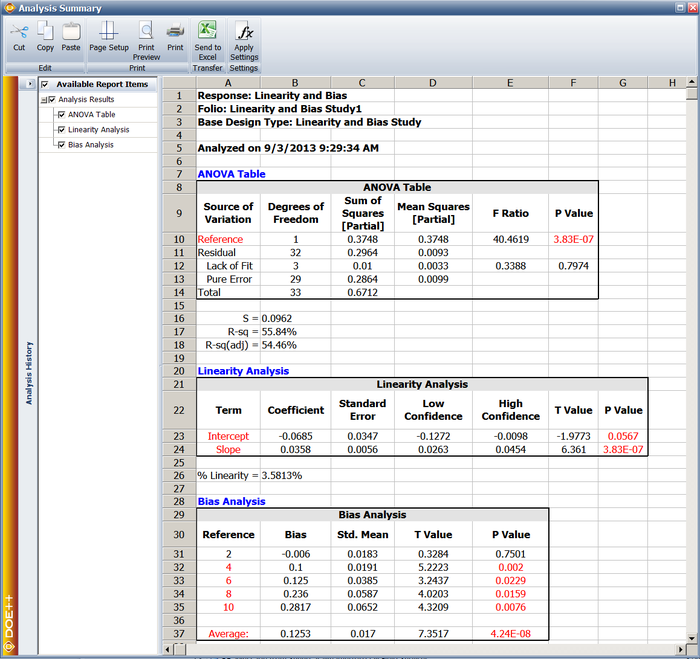
There are no clear cut-off values for what percent of linearity and bias are acceptable. Users should make their decision based on their engineering feeling or experience. The results from DOE++ is given in the following picture.


