Tensile Components Example

New format available! This reference is now available in a new format that offers faster page load, improved display for calculations and images and more targeted search.

As of January 2024, this Reliawiki page will not continue to be updated. Please update all links and bookmarks to the latest references at ALTA examples and ALTA reference examples.

---

A tensile component of a landing gear is put through an accelerated reliability test to determine whether the life goal would be achieved under the designed-in load. Fifteen units, N=15, are tested at three different shock loads. The component is designed for a peak shock load of 50 kips with an estimated return of 10% of the population by 10,000 cycles (or landings). Using the Inverse Power Law-Lognormal model, determine whether the design life is met.

The following table shows the data from the test.

Failure, in Cycles	Shock Load, kips
1855	73
2158	73
2425	73
2736	73
3206	73
614	95
770	95
781	95
890	95
1055	95
152	128
162	128
173	128
209	128
216	128

The data are entered into the ALTA standard folio, and the following parameters for the IPL-lognormal model are obtained:

[math]\displaystyle{ \begin{align} Std=\ & 0.179080 \\ K=\ & 8.953055E-13 \\ n=\ & 4.638882 \end{align} }[/math]

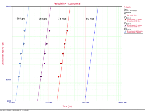
The following probability plot shows the plot at each test stress level (73 kips, 95 kips and 128 kips) and at the use stress level (50 kips). As you can see, there is a good agreement between the data and the fitted model.

The probability plot can be used to estimate the cycles-to failure for a 10% unreliability probability of failure. According to the plot, the cycles-to-failure is estimated to be [math]\displaystyle{ T(Q=0.10=10%)\approxeq 12,000 }[/math] landings. (By pressing SHIFT and clicking the plot, you can display the coordinates and read the value on the X axis that corresponds to a value of 10 in the Y axis.)

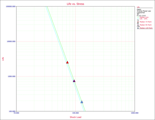
Another way to obtain life information is to use the Life vs. Stress plot to plot the life line that corresponds to the 10% unreliability. The following plot shows the life line for the 10% unreliability (the first line from the left). For a stress of 50 kips (X-axis) and for the 10% unreliability line, the cycles-to-failure can be obtained by reading the value on the Y-axis. Again, [math]\displaystyle{ T(0.1)\approxeq 12,000 }[/math] landings.

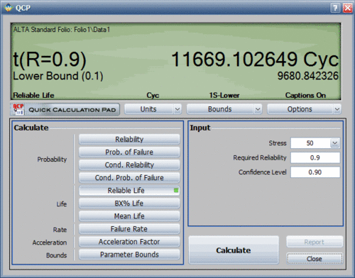
However, a more accurate way to obtain the information is to use the Quick Calculation Pad (QCP) in ALTA. Using the QCP, the life for a 10% probability of failure at 50 kips is estimated to be 11,669.1 landings, as shown next. Therefore, the design criterion of 10,000 landings is met.