Additional Analyses

The Repairable Systems Analysis Through Simulation chapter described the process of using discrete event simulation to perform basic system reliability, availability and maintainability analyses. This chapter discusses two additional types of analyses that can be performed with simulation: Throughput Analysis and Life Cycle Cost Analysis.

Throughput Analysis

In the prior sections, we concentrated on failure and repair actions of a system. In doing so, we viewed the system from a system/component up/down perspective. One could take this analysis a step further and consider system throughput as a part of the analysis. To define system throughput, assume that each component in the system processed (or made) something while operating. As an example, consider the case shown next with two components in series, each processing/producing 10 and 20 items per unit time (ipu) respectively.

In this case, the system configuration is not only the system's reliability-wise configuration but also its production/processing sequence. In other words, the first component processes/produces 10 ipu and the second component can process/produce up to 20 ipu. However, a block can only process/produce items it receives from the blocks before it. Therefore, the second component in this case is only receiving 10 ipu from the block before it. If we assume that neither component can fail, then the maximum items processed from this configuration would be 10 ipu. If the system were to operate for 100 time units, then the throughput of this system would be 1000 items, or [math]\displaystyle{ (100\cdot 10)\,\! }[/math].

Throughput Metrics and Terminology

In looking at throughput, one needs to define some terminology and metrics that will describe the behavior of the system and its components when doing such analyses. Some of the terminology used in BlockSim is given next.

• System Throughput: System throughput is the total amount of items processed/produced by the system over the defined period of time. In the two-component example, this is [math]\displaystyle{ 1000\,\! }[/math] items over [math]\displaystyle{ 100\,\! }[/math] time units.
  
• Component Throughput: The total amount of items processed or produced by each component (block). In the two-component example, this is [math]\displaystyle{ 1000\,\! }[/math] items each.
  
• Component Maximum Capacity: The maximum number of items that the component (block) could have processed/produced. This is simply the block's throughput rate multiplied by the run time. In the two-component example, this is [math]\displaystyle{ 100\cdot 10=1000\,\! }[/math] for the first component and [math]\displaystyle{ 100\cdot 20=2000\,\! }[/math] for the second component.
  
• Component Uptime Capacity: The maximum number of items the component could have processed/produced while it was up and running. In the two-component example, this is [math]\displaystyle{ 1000\,\! }[/math] for the first component and [math]\displaystyle{ 2000\,\! }[/math] for the second component, since we are assuming that the components cannot fail. If the components could fail, this number would be the component's uptime multiplied by its throughput rate.
  
• Component Excess Capacity: The additional amount a component could have processed/produced while up and running. In the two-component example, this is [math]\displaystyle{ 0\,\! }[/math] for the first component and [math]\displaystyle{ 1000\,\! }[/math] for the second component.
  
• Component Actual Utilization: The ratio of the component throughput and the component maximum capacity. In the two-component example, this is [math]\displaystyle{ 100%\,\! }[/math] for the first component and [math]\displaystyle{ 50%\,\! }[/math] for the second component.
  
• Component Uptime Utilization: The ratio of the component throughput and the component uptime capacity. In the two-component example, this is [math]\displaystyle{ 100%\,\! }[/math] for the first component and [math]\displaystyle{ 50%\,\! }[/math] for the second component. Note that if the components had failed and experienced downtime, this number would be different for each component.
  
• Backlog: Items that the component could not process are kept in a backlog. Depending on the settings, a backlog may or may not be processed when an opportunity arises. The available backlog metrics include:
  

• Component Backlog: The amount of a backlog present at the component at the end of the run (simulation).
  
• Component Processed Backlog: The amount of backlog processed by the component.
  
• Excess Backlog: Under specific settings in BlockSim, components can accept only a limited backlog. In these cases, a backlog that was rejected is stored in the Excess Backlog category.

Overview of Throughput Analysis

To examine throughput, consider the following scenarios.

Scenario 1

Consider the system shown in the figure below.

Blocks [math]\displaystyle{ A\,\! }[/math] through [math]\displaystyle{ I\,\! }[/math] produce a number of items per unit time as identified next to each letter (e.g., [math]\displaystyle{ A\,\! }[/math] : 100 implies [math]\displaystyle{ 100\,\! }[/math] items per time unit for [math]\displaystyle{ A\,\! }[/math] ). The connections shown in the RBD show the physical path of the items through the process (or production line). For the sake of simplicity, also assume that the blocks can never fail and that items are routed equally to each path.

This then implies that the following occurs over a single time unit:

• Unit [math]\displaystyle{ A\,\! }[/math] makes 100 items and routes 33.33 to [math]\displaystyle{ B\,\! }[/math], 33.33 to [math]\displaystyle{ C\,\! }[/math] and 33.33 to [math]\displaystyle{ D\,\! }[/math].
• In turn, [math]\displaystyle{ B\,\! }[/math], [math]\displaystyle{ C\,\! }[/math] and [math]\displaystyle{ D\,\! }[/math] route their 33.33 to [math]\displaystyle{ E\,\! }[/math], [math]\displaystyle{ F\,\! }[/math], [math]\displaystyle{ G\,\! }[/math] and [math]\displaystyle{ H\,\! }[/math] (8.33 to each path).
• [math]\displaystyle{ E\,\! }[/math], [math]\displaystyle{ F\,\! }[/math], [math]\displaystyle{ G\,\! }[/math] and [math]\displaystyle{ H\,\! }[/math] route 25 each to [math]\displaystyle{ I\,\! }[/math].
• [math]\displaystyle{ I\,\! }[/math] processes all 100.
• The system produces 100 items.

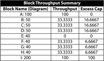
Thus, the following table would represent the throughput and excess capacity of each block after one time unit.

Run summary for Scenario 1.

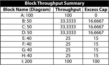
Scenario 2

Now consider the figure below where it is assumed that block [math]\displaystyle{ E\,\! }[/math] has failed.

Then:

• Unit [math]\displaystyle{ A\,\! }[/math] makes 100 items and routes 33.33 to [math]\displaystyle{ B\,\! }[/math], 33.33 to [math]\displaystyle{ C\,\! }[/math] and 33.33 to [math]\displaystyle{ D\,\! }[/math].
• In turn, [math]\displaystyle{ B\,\! }[/math], [math]\displaystyle{ C\,\! }[/math] and [math]\displaystyle{ D\,\! }[/math] route their 33.33 to [math]\displaystyle{ F\,\! }[/math], [math]\displaystyle{ G\,\! }[/math] and [math]\displaystyle{ H\,\! }[/math] (11.11 to each path that has an operating block at the end).
• [math]\displaystyle{ F\,\! }[/math], [math]\displaystyle{ G\,\! }[/math] and [math]\displaystyle{ H\,\! }[/math] route 33.33 each to [math]\displaystyle{ I\,\! }[/math].
• [math]\displaystyle{ I\,\! }[/math] processes all 100.
• he system produces 100 items.

A summary result table is shown next:

Run summary for Scenario 2.

Scenario 3

Finally, consider the figure below where both [math]\displaystyle{ E\,\! }[/math] and [math]\displaystyle{ H\,\! }[/math] have failed.

Then:

• Unit [math]\displaystyle{ A\,\! }[/math] makes 100 items and routes 33.33 to [math]\displaystyle{ B\,\! }[/math], 33.33 to [math]\displaystyle{ C\,\! }[/math] and 33.33 to [math]\displaystyle{ D\,\! }[/math].
• In turn, [math]\displaystyle{ B\,\! }[/math], [math]\displaystyle{ C\,\! }[/math] and [math]\displaystyle{ D\,\! }[/math] route their 33.33 to [math]\displaystyle{ F\,\! }[/math] and [math]\displaystyle{ G\,\! }[/math] (16.66 to each path that has an operating block at the end).
• [math]\displaystyle{ F\,\! }[/math] and [math]\displaystyle{ G\,\! }[/math] get 50 items each.
• [math]\displaystyle{ F\,\! }[/math] and [math]\displaystyle{ G\,\! }[/math] process and route 40 each (their maximum processing capacity) to [math]\displaystyle{ I\,\! }[/math]. Both have a backlog of 10 since they could not process all 50 items they received.
• [math]\displaystyle{ I\,\! }[/math] processes all 80.
• The system produces 80 items.

Run summary for Scenario 3.

Utilization summary for Scenario 3.

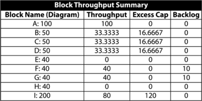
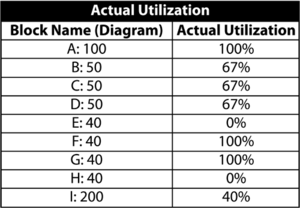
It can be easily seen that the bottlenecks in the system are the blocks [math]\displaystyle{ F\,\! }[/math] and [math]\displaystyle{ G\,\! }[/math].

Throughput Analysis Options

In BlockSim, specific throughput properties can be set for the blocks in the diagram.

Throughput: The number of items that the block can process per unit time.

Allocation: Specify the allocation scheme across multiple paths (i.e., equal or weighted). This option is shown in the figure below.

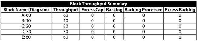
To explain these settings, consider the example shown in the above figure, which uses the same notation as before.

If the Weighted allocation across paths option is chosen, then the 60 items made by [math]\displaystyle{ A\,\! }[/math] will be allocated to [math]\displaystyle{ B\,\! }[/math], [math]\displaystyle{ C\,\! }[/math] and [math]\displaystyle{ D\,\! }[/math] based on their throughput capabilities. Specifically, the portion that each block will receive, [math]\displaystyle{ {{P}_{i}}\,\! }[/math], is:

[math]\displaystyle{ {{P}_{i}}=\frac{Throughpu{{t}_{i}}}{\underset{j=1}{\overset{N}{\mathop{\sum }}}\,Throughpu{{t}_{j}}} \ (eqn 1)\,\! }[/math]

The actual amount is then the (portion [math]\displaystyle{ \cdot \,\! }[/math] available units). In this case, the portion allocated to [math]\displaystyle{ B\,\! }[/math] is [math]\displaystyle{ \tfrac{10}{60},\,\! }[/math] the portion allocated to [math]\displaystyle{ C\,\! }[/math] is [math]\displaystyle{ \tfrac{20}{60}\,\! }[/math] and the portion allocated to [math]\displaystyle{ D\,\! }[/math] is [math]\displaystyle{ \tfrac{30}{60}\,\! }[/math]. When a total of 60 units is processed through [math]\displaystyle{ A\,\! }[/math], [math]\displaystyle{ B\,\! }[/math] will get 10, [math]\displaystyle{ C\,\! }[/math] will get 20 and [math]\displaystyle{ D\,\! }[/math] will get 30.

The results would then be as shown in the table below.

Throughput summary using weighted allocation across paths.

If the Allocate equal share to all paths option is chosen, then 20 units will be sent to [math]\displaystyle{ B\,\! }[/math], [math]\displaystyle{ C\,\! }[/math] and [math]\displaystyle{ D\,\! }[/math] regardless of their processing capacity, yielding the results shown in the table below.

Throughput summary using an equal allocation across paths.

Send units to failed blocks: Decide whether items should be sent to failed parts. If this option is not selected, the throughput units are allocated only to operational units. Otherwise, if this option is selected, units are also allocated to failed blocks and they become part of the failed block's backlog.

In the special case in which one or more blocks fail, causing a disruption in the path, and the Send units to failed blocks option is not selected, then the blocks that have a path to the failed block(s) will not be able to process any items, given the fact that they cannot be sent to the forward block. In this case, these blocks will keep all items received in their backlog. As an example, and using the figure below, if [math]\displaystyle{ E\,\! }[/math] is failed (and [math]\displaystyle{ E\,\! }[/math] cannot accept items in its backlog while failed), then [math]\displaystyle{ B\,\! }[/math], [math]\displaystyle{ C\,\! }[/math] and [math]\displaystyle{ D\,\! }[/math] cannot forward any items to it. Thus, they will not process any items sent to them from [math]\displaystyle{ A\,\! }[/math]. Items sent from [math]\displaystyle{ A\,\! }[/math] will be placed in the backlogs of items [math]\displaystyle{ B\,\! }[/math], [math]\displaystyle{ C\,\! }[/math] and [math]\displaystyle{ D.\,\! }[/math]

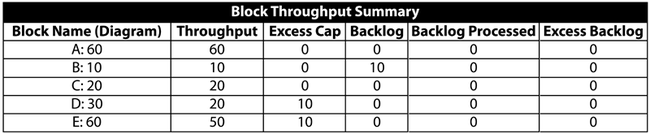
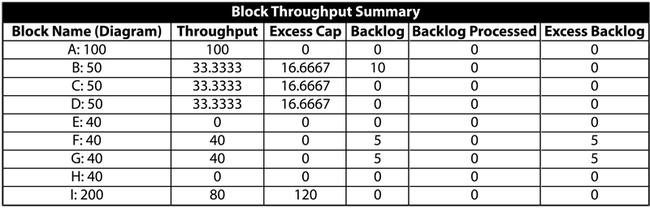
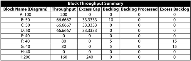
Process/Ignore backlog: Identify how a block handles backlog. A block can ignore or process backlog. Items that cannot be processed are kept in a backlog bin and are processed as needed.

Additionally, you can set the maximum number of items that can be stored in the backlog. When you choose to ignore the backlog, BlockSim will still report items that cannot be processed in the backlog column. However, it will let the backlog accumulate and never process it. In the case of a limited backlog, BlockSim will not accumulate more backlog than the maximum allowed and will discard all items sent to the block if they exceed its backlog capacity. It will keep count of the units that did not make it in the backlog in a category called Excess Backlog. To illustrate this, reconsider Scenario 3, but with both [math]\displaystyle{ F\,\! }[/math] and [math]\displaystyle{ G\,\! }[/math] having a limited backlog of 5. After a single time unit of operation, the results would be as shown in the tables below.

Scenario 3 summary with F and G having a limited blacklog and after one time unit.

Scenario 3 summary with F and G having a limited backlog and after two time units.

Note that the blocks will never be able to process the backlog in this example. However, if we were to observe the system for a longer operation time and through failures and repairs of the other blocks, there would be opportunities for the blocks to process their backlogs and catch up. It is very important to note that when simulating a system with failures and repairs in BlockSim, you must define the block as one that operates through system failure if you wish for backlog to be processed. If this option is not set, the block will not operate through system failure and thus will not be able to process any backlog items when components that cause system failure (from an RBD perspective) fail.

Throughput and Mirrored Blocks

Simulations that contain both mirrored blocks and throughput analysis behave in the following way:

System availability: All blocks within a mirror group will be considered the same block for system uptime/downtime analysis. This means that if the block fails, it will be considered a downed block everywhere that the mirrored block is found.

System throughput: The mirrored block throughput is NOT divided between each of the locations within the system diagram. Each instance of the mirrored block can process the amount of throughput assigned to the block.

Example

Imagine a system where block A and block C each have a throughput of 300 units/hour, while block B (mirrored block) and block D each have a throughput of 100 units/hour.

If all the blocks are operating, then the system throughput is 300 units/hour, as each instance of block B is able to handle 100 units/hour.

If block B is down, then the system throughput becomes 100 units/hour, as block B is considered down at both locations.

Variable Throughput

In many real-world cases throughput can change over time (i.e., throughput through a single component is not a constant but a function of time). The discussion in this chapter is devoted to cases of constant, non-variable throughput. BlockSim does model variable throughput using phase diagrams. These are discussed in Introduction to Reliability Phase Diagrams.

A Simple Throughput Analysis Example

The prior sections illustrated the basics concepts in throughput analysis. However, they did not take into account the reliability and maintenance properties of the blocks and the system. In a complete analysis, these would also need to be incorporated. The following simple example incorporates failures and repairs. Even though the example is trivial, the concepts presented here form the basis of throughput analysis in BlockSim. The principles remain the same no matter how complex the system.

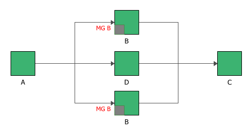
Consider the simple system shown in the figure below, but with [math]\displaystyle{ E\,\! }[/math] operating.

In addition, consider the following deterministic failure and repair characteristics:

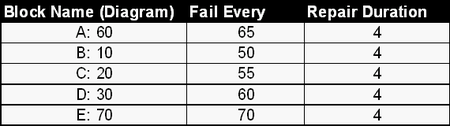
Also:

• Set all units to operate through system failure.
• Do not add spare part pools or crews (use defaults).
• Do not send items to failed units.
• Use a weighted allocation scheme.

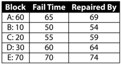
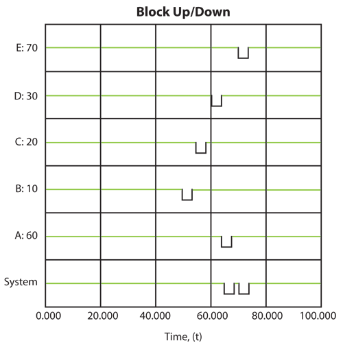
Event History: 0 to 100 Time Units

Then the system behavior from 0 to 100 time units is given in the table below. The system event history is as follows:

Once the system history has been established, we can examine the throughput behavior of this system from 0 to 100 by observing the sequence of events and their subsequent effect on system throughput.

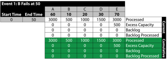
Event 1: B Fails at 50

• At 50, B fails.

• From 0 to 50, A processes [math]\displaystyle{ 50\cdot 60=3000\,\! }[/math] items.

• 500 are sent to B , 1000 to [math]\displaystyle{ C\,\! }[/math] and 1500 to [math]\displaystyle{ D\,\! }[/math]. There is no excess capacity at B , [math]\displaystyle{ C\,\! }[/math] or [math]\displaystyle{ D\,\! }[/math].

• B , [math]\displaystyle{ C\,\! }[/math] and [math]\displaystyle{ D\,\! }[/math] process and send 3000 items to [math]\displaystyle{ E\,\! }[/math]. Because the capacity of [math]\displaystyle{ E\,\! }[/math] is 3500, [math]\displaystyle{ E\,\! }[/math] now has an excess capacity of 500.

• The next table summarizes these results:

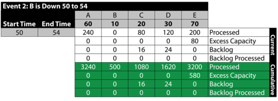
Event 2: B is Down 50 to 54

• From 50 to 54, B is down.

• A processes 240 items and sends 96 to [math]\displaystyle{ C\,\! }[/math] and 144 to [math]\displaystyle{ D\,\! }[/math].

• [math]\displaystyle{ D\,\! }[/math] and [math]\displaystyle{ C\,\! }[/math] can only process 80 and 120 respectively during this time. Thus, they get backlogs of 16 and 24 respectively.

• The 200 processed are sent to [math]\displaystyle{ E\,\! }[/math]. [math]\displaystyle{ E\,\! }[/math] has an excess capacity of 80 during this time period.

• The next table summarizes these results:

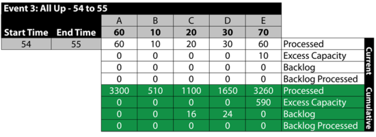
Event 3: All Up 54 to 55

The next table summarizes the results:

Event 4: [math]\displaystyle{ C\,\! }[/math] is Down 55 to 59

The next table summarizes the results:

Event 5: All Up 59 to 60

The next table summarizes the results:

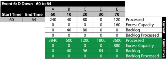
Event 6: [math]\displaystyle{ D\,\! }[/math] is Down 60 to 64
The next table summarizes the results:

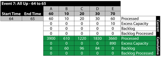
Event 7: All Up 64 to 65

The next table summarizes the results:

Event 8: A is Down 65 to 69

Between 65 and 69, A fails. This stops the flow of items in the system and provides an opportunity for the other blocks to process their backlogs. As an example, B processes 40 items from the 60 items in its backlog. Specifically:

Event 9: All Up 69 to 70

The next table summarizes the results:

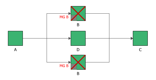
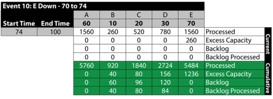
Event 10: [math]\displaystyle{ E\,\! }[/math] is Down 60 to 64

From 70 to 74, [math]\displaystyle{ E\,\! }[/math] is down. Because we specified that we will not send items to failed units, B , [math]\displaystyle{ C\,\! }[/math] and [math]\displaystyle{ D\,\! }[/math] receive items from A but they do not process them, since processing would require that items be sent to [math]\displaystyle{ E\,\! }[/math]. The items received by B , [math]\displaystyle{ C\,\! }[/math] and [math]\displaystyle{ D\,\! }[/math] are added to their respective backlogs. Furthermore, since they could have processed them if [math]\displaystyle{ E\,\! }[/math] had been up, all three blocks have an excess capacity for this period. Specifically:

It should be noted that if we had allowed items to be sent to failed blocks, B , [math]\displaystyle{ C\,\! }[/math] and [math]\displaystyle{ D\,\! }[/math] would have processed the items received and the backlog would have been at [math]\displaystyle{ E\,\! }[/math]. The rest of the time, all units are up.

Event 11: All Up 74 to 100

The next table summarizes the results:

Exploring the Results

BlockSim provides all of these results via the Simulation Results Explorer. The figure below shows the system throughput summary.

System level results present the total system throughput, which is 5484 items in this example. Additionally, the results include the uptime utilization of each component. The block level result summary, shown next, provides additional results for each item.

Finally, specific throughput results and metrics for each block are provided, as shown next.

Life Cycle Cost Analysis

A life cycle cost analysis involves the analysis of the costs of a system or a component over its entire life span. Typical costs for a system may include:

• Acquisition costs (or design and development costs).
• Operating costs:
  • Cost of failures.
  • Cost of repairs.
  • Cost for spares.
  • Downtime costs.
  • Loss of production.
• Disposal costs.

A complete life cycle cost (LCC) analysis may also include other costs, as well as other accounting/financial elements (such as discount rates, interest rates, depreciation, present value of money, etc.).

For the purpose of this reference, it is sufficient to say that if one has all the required cost values (inputs), then a complete LCC analysis can be performed easily in a spreadsheet, since it really involves summations of costs and perhaps some computations involving interest rates. With respect to the cost inputs for such an analysis, the costs involved are either deterministic (such as acquisition costs, disposal costs, etc.) or probabilistic (such as cost of failures, repairs, spares, downtime, etc.). Most of the probabilistic costs are directly related to the reliability and maintainability characteristics of the system.

The estimations of the associated probabilistic costs is the challenging aspect of LCC analysis. In the following example, we will look at using some of the cost inputs associated with BlockSim to obtain such costs.

Example: Obtaining Costs for an LCC Analysis

Consider the manufacturing line (or system) shown next.

The block properties, pool properties and crew properties are given in the following tables. All blocks identified with the same letter have the same properties (i.e., Blocks A = A1 and A2; Blocks B = B1, B2, B3 and B4; and Blocks C = C1, C2, C3 and C4).

This system was analyzed in BlockSim for a period of operation of 8,760 hours, or one year. 10,000 simulations were performed. The system overview is shown next.

Most of the variable costs of interest were obtained directly from BlockSim. The next figure shows the overall system costs.

From the summary, the total cost is $92,197.64. Note that an additional cost was defined in the problem statement that is not included in the summary. This cost, the operating cost per item per hour of operation, can be obtained by looking at the uptime of each block and then multiplying this by the cost per hour, as shown in the following table. Therefore, the total cost is [math]\displaystyle{ 92,197+313,813=\$406,010.\,\! }[/math]

If we also assume a revenue of $100 per unit produced, then the total revenue is our throughput multiplied by the per unit revenue, or [math]\displaystyle{ 31,685\cdot \$100=\$3,168,500.\,\! }[/math]