Additional Tools
Common Shape Parameter Likelihood Ratio Test
In order to assess the assumption of a common shape parameter among the data obtained at various stress levels, the likelihood ratio (LR) test can be utilized, as described in Nelson [28]. This test applies to any distribution with a shape parameter. In the case of ALTA, it applies to the Weibull and lognormal distributions. When Weibull is used as the underlying life distribution, the shape parameter, [math]\displaystyle{ \beta ,\,\! }[/math] is assumed to be constant across the different stress levels (i.e., stress independent). Similarly, [math]\displaystyle{ {{\sigma }_{{{T}'}}}\,\! }[/math], the parameter of the lognormal distribution is assumed to be constant across the different stress levels.
The likelihood ratio test is performed by first obtaining the LR test statistic, [math]\displaystyle{ T\,\! }[/math]. If the true shape parameters are equal, then the distribution of [math]\displaystyle{ T\,\! }[/math] is approximately chi-square with [math]\displaystyle{ n-1\,\! }[/math] degrees of freedom, where [math]\displaystyle{ n\,\! }[/math] is the number of test stress levels with two or more exact failure points. The LR test statistic, [math]\displaystyle{ T\,\! }[/math], is calculated as follows:
- [math]\displaystyle{ T=2({{\hat{\Lambda }}_{1}}+...+{{\hat{\Lambda }}_{n}}-{{\hat{\Lambda }}_{0}})\,\! }[/math]
where [math]\displaystyle{ \hat{\Lambda}_{1}, ..., \hat{\Lambda}_{n}\,\! }[/math] are the likelihood values obtained by fitting a separate distribution to the data from each of the [math]\displaystyle{ n\,\! }[/math] test stress levels (with two or more exact failure times). The likelihood value, [math]\displaystyle{ {{\hat{\Lambda }}_{0}},\,\! }[/math] is obtained by fitting a model with a common shape parameter and a separate scale parameter for each of the [math]\displaystyle{ n\,\! }[/math] stress levels, using indicator variables.
Once the LR statistic has been calculated, then:
- If [math]\displaystyle{ T\le {{\chi }^{2}}(1-\alpha ;n-1),\,\! }[/math] the [math]\displaystyle{ n\,\! }[/math] shape parameter estimates do not differ statistically significantly at the 100 [math]\displaystyle{ \alpha %\,\! }[/math] level.
- If [math]\displaystyle{ T\gt {{\chi }^{2}}(1-\alpha ;n-1),\,\! }[/math] the [math]\displaystyle{ n\,\! }[/math] shape parameter estimates differ statistically significantly at the 100 [math]\displaystyle{ \alpha %\,\! }[/math] level.
[math]\displaystyle{ {{\chi }^{2}}(1-\alpha ;n-1)\,\! }[/math] is the 100(1- [math]\displaystyle{ \alpha)\,\! }[/math] percentile of the chi-square distribution with [math]\displaystyle{ n-1\,\! }[/math] degrees of freedom.
Example: Likelihood Ratio Test Example
Consider the following times-to-failure data at three different stress levels.
| Stress | 406 K | 416 K | 426 K |
|---|---|---|---|
| Time Failed (hrs) | 248 | 164 | 92 |
| 456 | 176 | 105 | |
| 528 | 289 | 155 | |
| 731 | 319 | 184 | |
| 813 | 340 | 219 | |
| 543 | 235 |
The data set was analyzed using an Arrhenius-Weibull model. The analysis yields:
- [math]\displaystyle{ \widehat{\beta }=\ 2.965820\,\! }[/math]
- [math]\displaystyle{ \widehat{B}=\ 10,679.567542\,\! }[/math]
- [math]\displaystyle{ \widehat{C}=\ 2.396615\cdot {{10}^{-9}}\,\! }[/math]
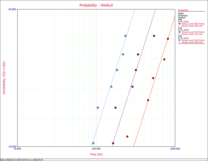
The assumption of a common [math]\displaystyle{ \beta \,\! }[/math] across the different stress levels can be visually assessed by using a probability plot. As you can see in the following plot, the plotted data from the different stress levels seem to be fairly parallel.
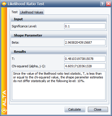
A better assessment can be made with the LR test, which can be performed using the Likelihood Ratio Test tool in ALTA. For example, in the following figure, the [math]\displaystyle{ \beta s\,\! }[/math] are compared for equality at the 10% level.
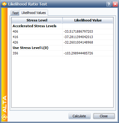
The LR test statistic, [math]\displaystyle{ T\,\! }[/math], is calculated to be 0.481. Therefore, [math]\displaystyle{ T=0.481\le 4.605={{\chi }^{2}}(0.9;2),\,\! }[/math] the [math]\displaystyle{ {\beta }'\,\! }[/math] s do not differ significantly at the 10% level. The individual likelihood values for each of the test stresses are shown next.
Tests of Comparison
It is often desirable to be able to compare two sets of accelerated life data in order to determine which of the data sets has a more favorable life distribution. The units from which the data are obtained could either be from two alternate designs, alternate manufacturers or alternate lots or assembly lines. Many methods are available in statistical literature for doing this when the units come from a complete sample, (i.e., a sample with no censoring). This process becomes a little more difficult when dealing with data sets that have censoring, or when trying to compare two data sets that have different distributions. In general, the problem boils down to that of being able to determine any statistically significant difference between the two samples of potentially censored data from two possibly different populations. This section discusses some of the methods that are applicable to censored data, and are available in ALTA.
Simple Plotting
One popular graphical method for making this determination involves plotting the data at a given stress level with confidence bounds and seeing whether the bounds overlap or separate at the point of interest. This can be effective for comparisons at a given point in time or a given reliability level, but it is difficult to assess the overall behavior of the two distributions, as the confidence bounds may overlap at some points and be far apart at others. This can be easily done using the overlay plot feature in ALTA.
Estimating [math]\displaystyle{ P\left[ {{t}_{2}}\ge {{t}_{1}} \right]\,\! }[/math] Using the Life Comparison Wizard
Another methodology, suggested by Gerald G. Brown and Herbert C. Rutemiller, is to estimate the probability of whether the times-to-failure of one population are better or worse than the times-to-failure of the second. The equation used to estimate this probability is given by:
- [math]\displaystyle{ P\left[ {{t}_{2}}\ge {{t}_{1}} \right]=\int_{0}^{\infty }{{f}_{1}}(t)\cdot {{R}_{2}}(t)\cdot dt\,\! }[/math]
where [math]\displaystyle{ {{f}_{1}}(t)\,\! }[/math] is the pdf of the first distribution and [math]\displaystyle{ {{R}_{2}}(t)\,\! }[/math] is the reliability function of the second distribution. The evaluation of the superior data set is based on whether this probability is smaller or greater than 0.50. If the probability is equal to 0.50, then is equivalent to saying that the two distributions are identical.
For example, consider two alternate designs, where X and Y represent the life test data from each design. If we simply wanted to choose the component with the higher reliability, we could simply select the component with the higher reliability at time [math]\displaystyle{ t\,\! }[/math]. However, if we wanted to design the product to be as long-lived as possible, we would want to calculate the probability that the entire distribution of one design is better than the other. The statement "the probability that X is greater than or equal to Y" can be interpreted as follows:
- If [math]\displaystyle{ P=0.50\,\! }[/math], then the statement is equivalent to saying that both X and Y are equal.
- If [math]\displaystyle{ P\lt 0.50\,\! }[/math] or, for example, [math]\displaystyle{ P=0.10\,\! }[/math], then the statement is equivalent to saying that [math]\displaystyle{ P=1-0.10=0.90\,\! }[/math], or Y is better than X with a 90% probability.
ALTA's Comparison Wizard allows you to perform such calculations. The comparison is performed at the given use stress levels of each data set, using the equation:
- [math]\displaystyle{ P\left[ {{t}_{2}}\ge {{t}_{1}} \right]=\int_{0}^{\infty }{{f}_{1}}(t,{{V}_{Use,1}})\cdot {{R}_{2}}(t,{{V}_{Use,2}})\cdot dt\,\! }[/math]
Degradation Analysis
Given that products are frequently being designed with higher reliabilities and developed in shorter amounts of time, even accelerated life testing is often not sufficient to yield reliability results in the desired timeframe. In some cases, it is possible to infer the reliability behavior of unfailed test samples with only the accumulated test time information and assumptions about the distribution. However, this generally leads to a great deal of uncertainty in the results. Another option in this situation is the use of degradation analysis. Degradation analysis involves the measurement and extrapolation of degradation or performance data that can be directly related to the presumed failure of the product in question. Many failure mechanisms can be directly linked to the degradation of part of the product, and degradation analysis allows the user to extrapolate to an assumed failure time based on the measurements of degradation or performance over time. To reduce testing time even further, tests can be performed at elevated stresses and the degradation at these elevated stresses can be measured resulting in a type of analysis known as accelerated degradation. In some cases, it is possible to directly measure the degradation over time, as with the wear of brake pads or with the propagation of crack size. In other cases, direct measurement of degradation might not be possible without invasive or destructive measurement techniques that would directly affect the subsequent performance of the product. In such cases, the degradation of the product can be estimated through the measurement of certain performance characteristics, such as using resistance to gauge the degradation of a dielectric material. In either case, however, it is necessary to be able to define a level of degradation or performance at which a failure is said to have occurred. With this failure level of performance defined, it is a relatively simple matter to use basic mathematical models to extrapolate the performance measurements over time to the point where the failure is said to occur. This is done at different stress levels, and therefore each time-to-failure is also associated with a corresponding stress level. Once the times-to-failure at the corresponding stress levels have been determined, it is merely a matter of analyzing the extrapolated failure times in the same manner as you would conventional accelerated time-to-failure data.
Once the level of failure (or the degradation level that would constitute a failure) is defined, the degradation for multiple units over time needs to be measured (with different groups of units being at different stress levels). As with conventional accelerated data, the amount of certainty in the results is directly related to the number of units being tested, the number of units at each stress level, as well as in the amount of overstressing with respect to the normal operating conditions. The performance or degradation of these units needs to be measured over time, either continuously or at predetermined intervals. Once this information has been recorded, the next task is to extrapolate the performance measurements to the defined failure level in order to estimate the failure time. ALTA allows the user to perform such analysis using a linear, exponential, power, logarithmic, Gompertz or Lloyd-Lipow model to perform this extrapolation. These models have the following forms:
where [math]\displaystyle{ y\,\! }[/math] represents the performance, [math]\displaystyle{ x\,\! }[/math] represents time, and [math]\displaystyle{ a\,\! }[/math] and [math]\displaystyle{ b\,\! }[/math] are model parameters to be solved for. Once the model parameters [math]\displaystyle{ {{a}_{i}}\,\! }[/math] and [math]\displaystyle{ {{b}_{i}}\,\! }[/math] (and [math]\displaystyle{ {{c}_{i}}\,\! }[/math] for Lloyd-Lipow) are estimated for each sample [math]\displaystyle{ i\,\! }[/math], a time, [math]\displaystyle{ {{x}_{i}},\,\! }[/math] can be extrapolated that corresponds to the defined level of failure [math]\displaystyle{ y\,\! }[/math]. The computed [math]\displaystyle{ {{x}_{i}}\,\! }[/math] can now be used as our times-to-failure for subsequent accelerated life data analysis. As with any sort of extrapolation, one must be careful not to extrapolate too far beyond the actual range of data in order to avoid large inaccuracies (modeling errors).
One may also define a censoring time past which no failure times are extrapolated. In practice, there is usually a rather narrow band in which this censoring time has any practical meaning. With a relatively low censoring time, no failure times will be extrapolated, which defeats the purpose of degradation analysis. A relatively high censoring time would occur after all of the theoretical failure times, thus being rendered meaningless. Nevertheless, certain situations may arise in which it is beneficial to be able to censor the accelerated degradation data.


