Bayesian-Weibull Analysis: Difference between revisions
Lisa Hacker (talk | contribs) No edit summary |
Lisa Hacker (talk | contribs) No edit summary |
||
| (19 intermediate revisions by 4 users not shown) | |||
| Line 1: | Line 1: | ||
{{template:LDABOOK|8.3|Bayesian-Weibull Analysis}} | |||
The Bayesian methods presented next are for the 2-parameter Weibull distribution. Bayesian concepts were introduced in [[Parameter Estimation]]. This model considers prior knowledge on the shape (<math>\beta\,\!</math>) parameter of the Weibull distribution when it is chosen to be fitted to a given set of data. There are many practical applications for this model, particularly when dealing with small sample sizes and some prior knowledge for the shape parameter is available. For example, when a test is performed, there is often a good understanding about the behavior of the failure mode under investigation, primarily through historical data. At the same time, most reliability tests are performed on a limited number of samples. Under these conditions, it would be very useful to use this prior knowledge with the goal of making more accurate predictions. A common approach for such scenarios is to use the 1-parameter Weibull distribution, but this approach is too deterministic, too absolute you may say (and you would be right). The Bayesian-Weibull model in Weibull++ (which is actually a true "WeiBayes" model, unlike the 1-parameter Weibull that is commonly referred to as such) offers an alternative to the 1-parameter Weibull, by including the variation and uncertainty that might have been observed in the past on the shape parameter. Applying Bayes's rule on the 2-parameter Weibull distribution and assuming the prior distributions of <math>\beta\,\!</math> and <math>\eta\,\!</math> are independent, we obtain the following posterior ''pdf'': | |||
::<math> f(\beta ,\eta |Data)=\dfrac{L(\beta ,\eta )\varphi (\beta )\varphi (\eta )}{ \int\nolimits_{0}^{\infty }\int\nolimits_{0}^{\infty }L(\beta ,\eta )\varphi (\beta )\varphi (\eta )d\eta d\beta } </math> | ::<math> f(\beta ,\eta |Data)=\dfrac{L(\beta ,\eta )\varphi (\beta )\varphi (\eta )}{ \int\nolimits_{0}^{\infty }\int\nolimits_{0}^{\infty }L(\beta ,\eta )\varphi (\beta )\varphi (\eta )d\eta d\beta } \,\!</math> | ||
In this model, < | In this model, <math>\eta\,\!</math> is assumed to follow a noninformative prior distribution with the density function <math> \varphi (\eta )=\dfrac{1}{\eta } \,\!</math>. This is called Jeffrey's prior, and is obtained by performing a logarithmic transformation on <math>\eta\,\!</math>. Specifically, since <math>\eta\,\!</math> is always positive, we can assume that ln(<math>\eta\,\!</math>) follows a uniform distribution, <math>U( -\infty, +\infty \,\!</math>). Applying Jeffrey's rule as given in Gelman et al. [[Appendix:_Life_Data_Analysis_References|[9]]] which says "in general, an approximate non-informative prior is taken proportional to the square root of Fisher's information," yields <math> \varphi (\eta )=\dfrac{1}{\eta }\,\!</math>. | ||
The prior distribution of < | The prior distribution of <math>\beta\,\!</math>, denoted as <math> \varphi (\beta )\,\!</math>, can be selected from the following distributions: normal, lognormal, exponential and uniform. The procedure of performing a Bayesian-Weibull analysis is as follows: | ||
*Collect the times-to-failure data. | :*Collect the times-to-failure data. | ||
*Specify a prior distribution for < | :*Specify a prior distribution for <math>\beta\,\!</math> (the prior for <math>\eta\,\!</math> is assumed to be <math>1/\beta\,\!</math>). | ||
*Obtain the posterior | :*Obtain the posterior ''pdf'' from the above equation. | ||
In other words, a distribution (the posterior ) is obtained, rather than a point estimate as in classical statistics (i.e., as in the parameter estimation methods described previously in this chapter). Therefore, if a point estimate needs to be reported, a point of the posterior | In other words, a distribution (the posterior ''pdf'') is obtained, rather than a point estimate as in classical statistics (i.e., as in the parameter estimation methods described previously in this chapter). Therefore, if a point estimate needs to be reported, a point of the posterior ''pdf'' needs to be calculated. Typical points of the posterior distribution used are the mean (expected value) or median. In Weibull++, both options are available and can be chosen from the ''Analysis'' page, under the ''Results As'' area, as shown next. | ||
[[Image:Weibull Distribution Wei-Bayesian for Choose Mean and Median.png|center|200px| ]] | |||
The expected value of <math>\beta\,\!</math> is obtained by: | |||
The expected value of < | |||
::<math> E(\beta )=\int\nolimits_{0}^{\infty }\int\nolimits_{0}^{\infty }\beta \cdot f(\beta ,\eta |Data)d\beta d\eta \,\!</math> | |||
Similarly, the expected value of <math>\eta\,\!</math> is obtained by: | |||
::<math> E(\eta )=\int\nolimits_{0}^{\infty }\int\nolimits_{0}^{\infty }\eta \cdot f(\beta ,\eta |Data)d\beta d\eta \,\!</math> | |||
The median points are obtained by solving the following equations for <math> \breve{\beta} \,\!</math> and <math> \breve{\eta} \,\!</math> respectively: | |||
::<math> \int\nolimits_{0}^{\infty }\int\nolimits_{0}^{\breve{\beta}}f(\beta ,\eta |Data)d\beta d\eta =0.5 \,\!</math> | |||
and: | |||
and | |||
::<math> \int\nolimits_{0}^{\breve{\eta}}\int\nolimits_{0}^{\infty }f(\beta ,\eta |Data)d\beta d\eta =0.5 \,\!</math> | |||
Of course, other points of the posterior distribution can be calculated as well. For example, one may want to calculate the 10th percentile of the joint posterior distribution (w.r.t. one of the parameters). The procedure for obtaining other points of the posterior distribution is similar to the one for obtaining the median values, where instead of 0.5 the percentage of interest is given. This procedure actually provides the confidence bounds on the parameters, which in the Bayesian framework are called ‘‘Credible Bounds.‘‘ However, since the engineering interpretation is the same, and to avoid confusion, we refer to them as confidence bounds in this reference and in Weibull++. | |||
As explained in | === Posterior Distributions for Functions of Parameters === | ||
As explained in [[Parameter Estimation]], in Bayesian analysis, all the functions of the parameters are distributed. In other words, a posterior distribution is obtained for functions such as reliability and failure rate, instead of point estimate as in classical statistics. Therefore, in order to obtain a point estimate for these functions, a point on the posterior distributions needs to be calculated. Again, the expected value (mean) or median value are used. It is important to note that the Median value is preferable and is the default in Weibull++. This is because the Median value always corresponds to the 50th percentile of the distribution. On the other hand, the Mean is not a fixed point on the distribution, which could cause issues, especially when comparing results across different data sets. | |||
'''pdf of the Times-to-Failure''' | |||
The posterior distribution of the failure time | The posterior distribution of the failure time <math>t\,\!</math> is given by: | ||
::<math> f(T|Data)=\int\nolimits_{0}^{\infty }\int\nolimits_{0}^{\infty }f(T,\beta ,\eta )f(\beta ,\eta |Data)d\eta d\beta </math> | ::<math> f(T|Data)=\int\nolimits_{0}^{\infty }\int\nolimits_{0}^{\infty }f(T,\beta ,\eta )f(\beta ,\eta |Data)d\eta d\beta \,\!</math> | ||
where: | where: | ||
::<math> f(T,\beta ,\eta )=\dfrac{\beta }{\eta }\left( \dfrac{T}{\eta }\right) ^{\beta -1}e^{-\left( \dfrac{T}{\eta }\right) ^{\beta }} </math> | ::<math> f(T,\beta ,\eta )=\dfrac{\beta }{\eta }\left( \dfrac{T}{\eta }\right) ^{\beta -1}e^{-\left( \dfrac{T}{\eta }\right) ^{\beta }} \,\!</math> | ||
For the | For the ''pdf'' of the times-to-failure, only the expected value is calculated and reported in Weibull++. | ||
'''Reliability''' | |||
In order to calculate the median value of the reliability function, we first need to obtain posterior | In order to calculate the median value of the reliability function, we first need to obtain posterior ''pdf'' of the reliability. Since <math>R(T)\,\!</math> is a function of <math>\beta\,\!</math>, the density functions of <math>\beta\,\!</math> and <math>R(T)\,\!</math> have the following relationship: | ||
::<math> \begin{align} f(R|Data,T)dR = & f(\beta |Data)d\beta)\\ | ::<math> \begin{align} f(R|Data,T)dR = & f(\beta |Data)d\beta)\\ | ||
= & (\int\nolimits_{0}^{\infty }f(\beta ,\eta |Data)d{\eta}) d{\beta} \\ | = & (\int\nolimits_{0}^{\infty }f(\beta ,\eta |Data)d{\eta}) d{\beta} \\ | ||
=& \dfrac{\int\nolimits_{0}^{\infty }L(\beta ,\eta )\varphi (\beta )\varphi (\eta )d\eta }{\int\nolimits_{0}^{\infty }\int\nolimits_{0}^{\infty }L(\beta ,\eta )\varphi (\beta )\varphi (\eta )d\eta d\beta }d\beta | =& \dfrac{\int\nolimits_{0}^{\infty }L(\beta ,\eta )\varphi (\beta )\varphi (\eta )d\eta }{\int\nolimits_{0}^{\infty }\int\nolimits_{0}^{\infty }L(\beta ,\eta )\varphi (\beta )\varphi (\eta )d\eta d\beta }d\beta | ||
\end{align} | \end{align}\,\!</math> | ||
</math> | |||
The median value of the reliability is obtained by solving the following equation w.r.t. <math> \breve{R}: \,\!</math> | |||
::<math> \int\nolimits_{0}^{\breve{R}}f(R|Data,T)dR=0.5 \,\!</math> | |||
The expected value of the reliability at time <math>t\,\!</math> is given by: | |||
::<math> R(T|Data)=\int\nolimits_{0}^{\infty }\int\nolimits_{0}^{\infty }R(T,\beta ,\eta )f(\beta ,\eta |Data)d\eta d\beta \,\!</math> | |||
where: | |||
::<math> R(T,\beta ,\eta )=e^{-\left( \dfrac{T}{\eta }\right) ^{^{\beta }}} </math> | ::<math> R(T,\beta ,\eta )=e^{-\left( \dfrac{T}{\eta }\right) ^{^{\beta }}} \,\!</math> | ||
<br> | <br> | ||
'''Failure Rate''' | |||
The failure rate at time is given by: | The failure rate at time is given by: | ||
::<math> \lambda (T|Data)=\dfrac{\int\nolimits_{0}^{\infty }\int\nolimits_{0}^{\infty }\lambda (T,\beta ,\eta )L(\beta ,\eta )\varphi (\eta )\varphi (\beta )d\eta d\beta }{\int\nolimits_{0}^{\infty }\int\nolimits_{0}^{\infty }L(\beta ,\eta )\varphi (\eta )\varphi (\beta )d\eta d\beta } </math> | ::<math> \lambda (T|Data)=\dfrac{\int\nolimits_{0}^{\infty }\int\nolimits_{0}^{\infty }\lambda (T,\beta ,\eta )L(\beta ,\eta )\varphi (\eta )\varphi (\beta )d\eta d\beta }{\int\nolimits_{0}^{\infty }\int\nolimits_{0}^{\infty }L(\beta ,\eta )\varphi (\eta )\varphi (\beta )d\eta d\beta } \,\!</math> | ||
where: | where: | ||
::<math> \lambda (T,\beta ,\eta )=\dfrac{\beta }{\eta }\left( \dfrac{T}{\eta }\right) ^{\beta -1} </math> | ::<math> \lambda (T,\beta ,\eta )=\dfrac{\beta }{\eta }\left( \dfrac{T}{\eta }\right) ^{\beta -1} \,\!</math> | ||
<br> | <br> | ||
== | === Bounds on Reliability for Bayesian-Weibull=== | ||
The confidence bounds calculation under the Bayesian-Weibull analysis is very similar to the Bayesian Confidence Bounds method described in the previous section, with the exception that in the case of the Bayesian-Weibull Analysis the specified prior of <math>\beta\,\!</math> is considered instead of an non-informative prior. The Bayesian one-sided upper bound estimate for <math>R(T)\,\!</math> is given by: | |||
::<math> \int\nolimits_{0}^{R_{U}(T)}f(R|Data,t)dR=CL \,\!</math> | |||
Using the posterior distribution, the following is obtained: | |||
::<math> \dfrac{\int\nolimits_{0}^{\infty }\int\nolimits_{t\exp (-\dfrac{\ln (-\ln R_{U})}{\beta })}^{\infty }L(\beta ,\eta )\varphi (\beta )\varphi (\eta )d\eta d\beta }{\int\nolimits_{0}^{\infty }\int\nolimits_{0}^{\infty }L(\beta ,\eta )\varphi (\beta )\varphi (\eta )d\eta d\beta }=CL \,\!</math> | |||
The above equation can be solved for <math>{{R}_{U}}(t)\,\!</math>. The Bayesian one-sided lower bound estimate for <math> \ R(t) \,\!</math> is given by: | |||
::<math> \int\nolimits_{0}^{R_{L}(t)}f(R|Data,t)dR=1-CL \,\!</math> | |||
: | Using the posterior distribution, the following is obtained: | ||
::<math> \dfrac{\int\nolimits_{0}^{\infty }\int\nolimits_{0}^{T\exp (-\dfrac{\ln (-\ln R_{L})}{\beta })}L(\beta ,\eta )\varphi (\beta )\varphi (\eta )d\eta d\beta }{\int\nolimits_{0}^{\infty }\int\nolimits_{0}^{\infty }L(\beta ,\eta )\varphi (\beta )\varphi (\eta )d\eta d\beta }=1-CL \,\!</math> | |||
The above equation can be solved for <math>{{R}_{L}}(t)\,\!</math>. The Bayesian two-sided bounds estimate for <math>R(t)\,\!</math> is given by: | |||
::<math> \int\nolimits_{R_{L}(t)}^{R_{U}(t)}f(R|Data,t)dR=CL \,\!</math> which is equivalent to: | |||
::<math> | ::<math> \int\nolimits_{0}^{R_{U}(t)}f(R|Data,t)dR=(1+CL)/2 \,\!</math> | ||
and: | |||
::<math> \int\nolimits_{ | ::<math> \int\nolimits_{0}^{R_{L}(t)}f(R|Data,T)dR=(1-CL)/2 \,\!</math> | ||
Using the same method for one-sided bounds, <math>{{R}_{U}}(t)\,\!</math> and <math>{{R}_{L}}(t)\,\!</math> can be computed. | |||
=== Bounds on Time for Bayesian-Weibull=== | |||
Following the same procedure described for bounds on Reliability, the bounds of time <math>t\,\!</math> can be calculated, given <math>R\,\!</math>. The Bayesian one-sided upper bound estimate for <math>t(R)\,\!</math> is given by: | |||
::<math> \int\nolimits_{0}^{ | ::<math> \int\nolimits_{0}^{T_{U}(R)}f(T|Data,R)dT=CL \,\!</math> | ||
Using the | Using the posterior distribution, the following is obtained: | ||
::<math> \dfrac{\int\nolimits_{0}^{\infty }\int\nolimits_{0}^{T_{U}\exp (-\dfrac{\ln (-\ln R)}{\beta })}L(\beta ,\eta )\varphi (\beta )\varphi (\eta )d\eta d\beta }{\int\nolimits_{0}^{\infty }\int\nolimits_{0}^{\infty }L(\beta ,\eta )\varphi (\beta )\varphi (\eta )d\eta d\beta }=CL </math> | ::<math> \dfrac{\int\nolimits_{0}^{\infty }\int\nolimits_{0}^{T_{U}\exp (-\dfrac{\ln (-\ln R)}{\beta })}L(\beta ,\eta )\varphi (\beta )\varphi (\eta )d\eta d\beta }{\int\nolimits_{0}^{\infty }\int\nolimits_{0}^{\infty }L(\beta ,\eta )\varphi (\beta )\varphi (\eta )d\eta d\beta }=CL \,\!</math> | ||
The above equation can be solved for <math>{{T}_{U}}(R)\,\!</math>. The Bayesian one-sided lower bound estimate for <math>T(R)\,\!</math> is given by: | |||
::<math> \int\nolimits_{0}^{T_{L}(R)}f(T|Data,R)dT=1-CL </math> | ::<math> \int\nolimits_{0}^{T_{L}(R)}f(T|Data,R)dT=1-CL \,\!</math> | ||
or: | or: | ||
::<math> \dfrac{\int\nolimits_{0}^{\infty }\int\nolimits_{T_{L}\exp (\dfrac{-\ln (-\ln R)}{\beta })}^{\infty }L(\beta ,\eta )\varphi (\beta )\varphi (\eta )d\eta d\beta }{\int\nolimits_{0}^{\infty }\int\nolimits_{0}^{\infty }L(\beta ,\eta )\varphi (\beta )\varphi (\eta )d\eta d\beta }=CL </math> | ::<math> \dfrac{\int\nolimits_{0}^{\infty }\int\nolimits_{T_{L}\exp (\dfrac{-\ln (-\ln R)}{\beta })}^{\infty }L(\beta ,\eta )\varphi (\beta )\varphi (\eta )d\eta d\beta }{\int\nolimits_{0}^{\infty }\int\nolimits_{0}^{\infty }L(\beta ,\eta )\varphi (\beta )\varphi (\eta )d\eta d\beta }=CL \,\!</math> | ||
The above equation can be solved for <math>{{T}_{L}}(R)\,\!</math>. The Bayesian two-sided lower bounds estimate for <math>T(R)\,\!</math> is: | |||
::<math> \int\nolimits_{T_{L}(R)}^{T_{U}(R)}f(T|Data,R)dT=CL </math> | ::<math> \int\nolimits_{T_{L}(R)}^{T_{U}(R)}f(T|Data,R)dT=CL \,\!</math> | ||
which is equivalent to: | which is equivalent to: | ||
::<math> \int\nolimits_{0}^{T_{U}(R)}f(T|Data,R)dT=(1+CL)/2 </math> | ::<math> \int\nolimits_{0}^{T_{U}(R)}f(T|Data,R)dT=(1+CL)/2 \,\!</math> | ||
and: | and: | ||
::<math> \int\nolimits_{0}^{T_{L}(R)}f(T|Data,R)dT=(1-CL)/2 </math> | ::<math> \int\nolimits_{0}^{T_{L}(R)}f(T|Data,R)dT=(1-CL)/2 \,\!</math> | ||
<br> | <br> | ||
===Bayesian-Weibull Example=== | |||
{{:Bayesian-Weibull_Lognormal_Prior Example}} | |||
{ | |||
Latest revision as of 00:13, 9 March 2023
The Bayesian methods presented next are for the 2-parameter Weibull distribution. Bayesian concepts were introduced in Parameter Estimation. This model considers prior knowledge on the shape ([math]\displaystyle{ \beta\,\! }[/math]) parameter of the Weibull distribution when it is chosen to be fitted to a given set of data. There are many practical applications for this model, particularly when dealing with small sample sizes and some prior knowledge for the shape parameter is available. For example, when a test is performed, there is often a good understanding about the behavior of the failure mode under investigation, primarily through historical data. At the same time, most reliability tests are performed on a limited number of samples. Under these conditions, it would be very useful to use this prior knowledge with the goal of making more accurate predictions. A common approach for such scenarios is to use the 1-parameter Weibull distribution, but this approach is too deterministic, too absolute you may say (and you would be right). The Bayesian-Weibull model in Weibull++ (which is actually a true "WeiBayes" model, unlike the 1-parameter Weibull that is commonly referred to as such) offers an alternative to the 1-parameter Weibull, by including the variation and uncertainty that might have been observed in the past on the shape parameter. Applying Bayes's rule on the 2-parameter Weibull distribution and assuming the prior distributions of [math]\displaystyle{ \beta\,\! }[/math] and [math]\displaystyle{ \eta\,\! }[/math] are independent, we obtain the following posterior pdf:
- [math]\displaystyle{ f(\beta ,\eta |Data)=\dfrac{L(\beta ,\eta )\varphi (\beta )\varphi (\eta )}{ \int\nolimits_{0}^{\infty }\int\nolimits_{0}^{\infty }L(\beta ,\eta )\varphi (\beta )\varphi (\eta )d\eta d\beta } \,\! }[/math]
In this model, [math]\displaystyle{ \eta\,\! }[/math] is assumed to follow a noninformative prior distribution with the density function [math]\displaystyle{ \varphi (\eta )=\dfrac{1}{\eta } \,\! }[/math]. This is called Jeffrey's prior, and is obtained by performing a logarithmic transformation on [math]\displaystyle{ \eta\,\! }[/math]. Specifically, since [math]\displaystyle{ \eta\,\! }[/math] is always positive, we can assume that ln([math]\displaystyle{ \eta\,\! }[/math]) follows a uniform distribution, [math]\displaystyle{ U( -\infty, +\infty \,\! }[/math]). Applying Jeffrey's rule as given in Gelman et al. [9] which says "in general, an approximate non-informative prior is taken proportional to the square root of Fisher's information," yields [math]\displaystyle{ \varphi (\eta )=\dfrac{1}{\eta }\,\! }[/math].
The prior distribution of [math]\displaystyle{ \beta\,\! }[/math], denoted as [math]\displaystyle{ \varphi (\beta )\,\! }[/math], can be selected from the following distributions: normal, lognormal, exponential and uniform. The procedure of performing a Bayesian-Weibull analysis is as follows:
- Collect the times-to-failure data.
- Specify a prior distribution for [math]\displaystyle{ \beta\,\! }[/math] (the prior for [math]\displaystyle{ \eta\,\! }[/math] is assumed to be [math]\displaystyle{ 1/\beta\,\! }[/math]).
- Obtain the posterior pdf from the above equation.
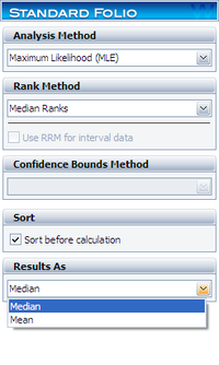
In other words, a distribution (the posterior pdf) is obtained, rather than a point estimate as in classical statistics (i.e., as in the parameter estimation methods described previously in this chapter). Therefore, if a point estimate needs to be reported, a point of the posterior pdf needs to be calculated. Typical points of the posterior distribution used are the mean (expected value) or median. In Weibull++, both options are available and can be chosen from the Analysis page, under the Results As area, as shown next.
The expected value of [math]\displaystyle{ \beta\,\! }[/math] is obtained by:
- [math]\displaystyle{ E(\beta )=\int\nolimits_{0}^{\infty }\int\nolimits_{0}^{\infty }\beta \cdot f(\beta ,\eta |Data)d\beta d\eta \,\! }[/math]
Similarly, the expected value of [math]\displaystyle{ \eta\,\! }[/math] is obtained by:
- [math]\displaystyle{ E(\eta )=\int\nolimits_{0}^{\infty }\int\nolimits_{0}^{\infty }\eta \cdot f(\beta ,\eta |Data)d\beta d\eta \,\! }[/math]
The median points are obtained by solving the following equations for [math]\displaystyle{ \breve{\beta} \,\! }[/math] and [math]\displaystyle{ \breve{\eta} \,\! }[/math] respectively:
- [math]\displaystyle{ \int\nolimits_{0}^{\infty }\int\nolimits_{0}^{\breve{\beta}}f(\beta ,\eta |Data)d\beta d\eta =0.5 \,\! }[/math]
and:
- [math]\displaystyle{ \int\nolimits_{0}^{\breve{\eta}}\int\nolimits_{0}^{\infty }f(\beta ,\eta |Data)d\beta d\eta =0.5 \,\! }[/math]
Of course, other points of the posterior distribution can be calculated as well. For example, one may want to calculate the 10th percentile of the joint posterior distribution (w.r.t. one of the parameters). The procedure for obtaining other points of the posterior distribution is similar to the one for obtaining the median values, where instead of 0.5 the percentage of interest is given. This procedure actually provides the confidence bounds on the parameters, which in the Bayesian framework are called ‘‘Credible Bounds.‘‘ However, since the engineering interpretation is the same, and to avoid confusion, we refer to them as confidence bounds in this reference and in Weibull++.
Posterior Distributions for Functions of Parameters
As explained in Parameter Estimation, in Bayesian analysis, all the functions of the parameters are distributed. In other words, a posterior distribution is obtained for functions such as reliability and failure rate, instead of point estimate as in classical statistics. Therefore, in order to obtain a point estimate for these functions, a point on the posterior distributions needs to be calculated. Again, the expected value (mean) or median value are used. It is important to note that the Median value is preferable and is the default in Weibull++. This is because the Median value always corresponds to the 50th percentile of the distribution. On the other hand, the Mean is not a fixed point on the distribution, which could cause issues, especially when comparing results across different data sets.
pdf of the Times-to-Failure
The posterior distribution of the failure time [math]\displaystyle{ t\,\! }[/math] is given by:
- [math]\displaystyle{ f(T|Data)=\int\nolimits_{0}^{\infty }\int\nolimits_{0}^{\infty }f(T,\beta ,\eta )f(\beta ,\eta |Data)d\eta d\beta \,\! }[/math]
where:
- [math]\displaystyle{ f(T,\beta ,\eta )=\dfrac{\beta }{\eta }\left( \dfrac{T}{\eta }\right) ^{\beta -1}e^{-\left( \dfrac{T}{\eta }\right) ^{\beta }} \,\! }[/math]
For the pdf of the times-to-failure, only the expected value is calculated and reported in Weibull++.
Reliability
In order to calculate the median value of the reliability function, we first need to obtain posterior pdf of the reliability. Since [math]\displaystyle{ R(T)\,\! }[/math] is a function of [math]\displaystyle{ \beta\,\! }[/math], the density functions of [math]\displaystyle{ \beta\,\! }[/math] and [math]\displaystyle{ R(T)\,\! }[/math] have the following relationship:
- [math]\displaystyle{ \begin{align} f(R|Data,T)dR = & f(\beta |Data)d\beta)\\ = & (\int\nolimits_{0}^{\infty }f(\beta ,\eta |Data)d{\eta}) d{\beta} \\ =& \dfrac{\int\nolimits_{0}^{\infty }L(\beta ,\eta )\varphi (\beta )\varphi (\eta )d\eta }{\int\nolimits_{0}^{\infty }\int\nolimits_{0}^{\infty }L(\beta ,\eta )\varphi (\beta )\varphi (\eta )d\eta d\beta }d\beta \end{align}\,\! }[/math]
The median value of the reliability is obtained by solving the following equation w.r.t. [math]\displaystyle{ \breve{R}: \,\! }[/math]
- [math]\displaystyle{ \int\nolimits_{0}^{\breve{R}}f(R|Data,T)dR=0.5 \,\! }[/math]
The expected value of the reliability at time [math]\displaystyle{ t\,\! }[/math] is given by:
- [math]\displaystyle{ R(T|Data)=\int\nolimits_{0}^{\infty }\int\nolimits_{0}^{\infty }R(T,\beta ,\eta )f(\beta ,\eta |Data)d\eta d\beta \,\! }[/math]
where:
- [math]\displaystyle{ R(T,\beta ,\eta )=e^{-\left( \dfrac{T}{\eta }\right) ^{^{\beta }}} \,\! }[/math]
Failure Rate
The failure rate at time is given by:
- [math]\displaystyle{ \lambda (T|Data)=\dfrac{\int\nolimits_{0}^{\infty }\int\nolimits_{0}^{\infty }\lambda (T,\beta ,\eta )L(\beta ,\eta )\varphi (\eta )\varphi (\beta )d\eta d\beta }{\int\nolimits_{0}^{\infty }\int\nolimits_{0}^{\infty }L(\beta ,\eta )\varphi (\eta )\varphi (\beta )d\eta d\beta } \,\! }[/math]
where:
- [math]\displaystyle{ \lambda (T,\beta ,\eta )=\dfrac{\beta }{\eta }\left( \dfrac{T}{\eta }\right) ^{\beta -1} \,\! }[/math]
Bounds on Reliability for Bayesian-Weibull
The confidence bounds calculation under the Bayesian-Weibull analysis is very similar to the Bayesian Confidence Bounds method described in the previous section, with the exception that in the case of the Bayesian-Weibull Analysis the specified prior of [math]\displaystyle{ \beta\,\! }[/math] is considered instead of an non-informative prior. The Bayesian one-sided upper bound estimate for [math]\displaystyle{ R(T)\,\! }[/math] is given by:
- [math]\displaystyle{ \int\nolimits_{0}^{R_{U}(T)}f(R|Data,t)dR=CL \,\! }[/math]
Using the posterior distribution, the following is obtained:
- [math]\displaystyle{ \dfrac{\int\nolimits_{0}^{\infty }\int\nolimits_{t\exp (-\dfrac{\ln (-\ln R_{U})}{\beta })}^{\infty }L(\beta ,\eta )\varphi (\beta )\varphi (\eta )d\eta d\beta }{\int\nolimits_{0}^{\infty }\int\nolimits_{0}^{\infty }L(\beta ,\eta )\varphi (\beta )\varphi (\eta )d\eta d\beta }=CL \,\! }[/math]
The above equation can be solved for [math]\displaystyle{ {{R}_{U}}(t)\,\! }[/math]. The Bayesian one-sided lower bound estimate for [math]\displaystyle{ \ R(t) \,\! }[/math] is given by:
- [math]\displaystyle{ \int\nolimits_{0}^{R_{L}(t)}f(R|Data,t)dR=1-CL \,\! }[/math]
Using the posterior distribution, the following is obtained:
- [math]\displaystyle{ \dfrac{\int\nolimits_{0}^{\infty }\int\nolimits_{0}^{T\exp (-\dfrac{\ln (-\ln R_{L})}{\beta })}L(\beta ,\eta )\varphi (\beta )\varphi (\eta )d\eta d\beta }{\int\nolimits_{0}^{\infty }\int\nolimits_{0}^{\infty }L(\beta ,\eta )\varphi (\beta )\varphi (\eta )d\eta d\beta }=1-CL \,\! }[/math]
The above equation can be solved for [math]\displaystyle{ {{R}_{L}}(t)\,\! }[/math]. The Bayesian two-sided bounds estimate for [math]\displaystyle{ R(t)\,\! }[/math] is given by:
- [math]\displaystyle{ \int\nolimits_{R_{L}(t)}^{R_{U}(t)}f(R|Data,t)dR=CL \,\! }[/math] which is equivalent to:
- [math]\displaystyle{ \int\nolimits_{0}^{R_{U}(t)}f(R|Data,t)dR=(1+CL)/2 \,\! }[/math]
and:
- [math]\displaystyle{ \int\nolimits_{0}^{R_{L}(t)}f(R|Data,T)dR=(1-CL)/2 \,\! }[/math]
Using the same method for one-sided bounds, [math]\displaystyle{ {{R}_{U}}(t)\,\! }[/math] and [math]\displaystyle{ {{R}_{L}}(t)\,\! }[/math] can be computed.
Bounds on Time for Bayesian-Weibull
Following the same procedure described for bounds on Reliability, the bounds of time [math]\displaystyle{ t\,\! }[/math] can be calculated, given [math]\displaystyle{ R\,\! }[/math]. The Bayesian one-sided upper bound estimate for [math]\displaystyle{ t(R)\,\! }[/math] is given by:
- [math]\displaystyle{ \int\nolimits_{0}^{T_{U}(R)}f(T|Data,R)dT=CL \,\! }[/math]
Using the posterior distribution, the following is obtained:
- [math]\displaystyle{ \dfrac{\int\nolimits_{0}^{\infty }\int\nolimits_{0}^{T_{U}\exp (-\dfrac{\ln (-\ln R)}{\beta })}L(\beta ,\eta )\varphi (\beta )\varphi (\eta )d\eta d\beta }{\int\nolimits_{0}^{\infty }\int\nolimits_{0}^{\infty }L(\beta ,\eta )\varphi (\beta )\varphi (\eta )d\eta d\beta }=CL \,\! }[/math]
The above equation can be solved for [math]\displaystyle{ {{T}_{U}}(R)\,\! }[/math]. The Bayesian one-sided lower bound estimate for [math]\displaystyle{ T(R)\,\! }[/math] is given by:
- [math]\displaystyle{ \int\nolimits_{0}^{T_{L}(R)}f(T|Data,R)dT=1-CL \,\! }[/math]
or:
- [math]\displaystyle{ \dfrac{\int\nolimits_{0}^{\infty }\int\nolimits_{T_{L}\exp (\dfrac{-\ln (-\ln R)}{\beta })}^{\infty }L(\beta ,\eta )\varphi (\beta )\varphi (\eta )d\eta d\beta }{\int\nolimits_{0}^{\infty }\int\nolimits_{0}^{\infty }L(\beta ,\eta )\varphi (\beta )\varphi (\eta )d\eta d\beta }=CL \,\! }[/math]
The above equation can be solved for [math]\displaystyle{ {{T}_{L}}(R)\,\! }[/math]. The Bayesian two-sided lower bounds estimate for [math]\displaystyle{ T(R)\,\! }[/math] is:
- [math]\displaystyle{ \int\nolimits_{T_{L}(R)}^{T_{U}(R)}f(T|Data,R)dT=CL \,\! }[/math]
which is equivalent to:
- [math]\displaystyle{ \int\nolimits_{0}^{T_{U}(R)}f(T|Data,R)dT=(1+CL)/2 \,\! }[/math]
and:
- [math]\displaystyle{ \int\nolimits_{0}^{T_{L}(R)}f(T|Data,R)dT=(1-CL)/2 \,\! }[/math]
Bayesian-Weibull Example
A manufacturer has tested prototypes of a modified product. The test was terminated at 2,000 hours, with only 2 failures observed from a sample size of 18. The following table shows the data.
| Number of State | State of F or S | State End Time |
|---|---|---|
| 1 | F | 1180 |
| 1 | F | 1842 |
| 16 | S | 2000 |
Because of the lack of failure data in the prototype testing, the manufacturer decided to use information gathered from prior tests on this product to increase the confidence in the results of the prototype testing. This decision was made because failure analysis indicated that the failure mode of the two failures is the same as the one that was observed in previous tests. In other words, it is expected that the shape of the distribution (beta) hasn't changed, but hopefully the scale (eta) has, indicating longer life. The 2-parameter Weibull distribution was used to model all prior tests results. The estimated beta ([math]\displaystyle{ \beta\,\! }[/math]) parameters of the prior test results are as follows:
| Betas Obtained for Similar Mode |
|---|
| 1.7 |
| 2.1 |
| 2.4 |
| 3.1 |
| 3.5 |
Solution
First, in order to fit the data to a Bayesian-Weibull model, a prior distribution for beta needs to be determined. Based on the beta values in the prior tests, the prior distribution for beta is found to be a lognormal distribution with [math]\displaystyle{ \mu = 0.9064\,\! }[/math], [math]\displaystyle{ \sigma = 0.3325\,\! }[/math]. (The values of the parameters can be obtained by entering the beta values into a Weibull++ standard folio and analyzing it using the lognormal distribution and the RRX analysis method.)
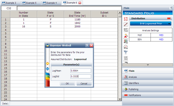
Next, enter the data from the prototype testing into a standard folio. On the control panel, choose the Bayesian-Weibull > B-W Lognormal Prior distribution. Click Calculate and enter the parameters of the lognormal distribution, as shown next.
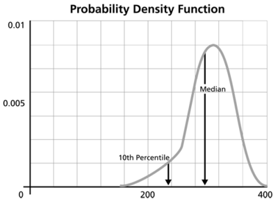
Click OK. The result is Beta (Median) = 2.361219 and Eta (Median) = 5321.631912 (by default Weibull++ returns the median values of the posterior distribution). Suppose that the reliability at 3,000 hours is the metric of interest in this example. Using the QCP, the reliability is calculated to be 76.97% at 3,000 hours. The following picture depicts the posterior pdf plot of the reliability at 3,000, with the corresponding median value as well as the 10th percentile value. The 10th percentile constitutes the 90% lower 1-sided bound on the reliability at 3,000 hours, which is calculated to be 50.77%.
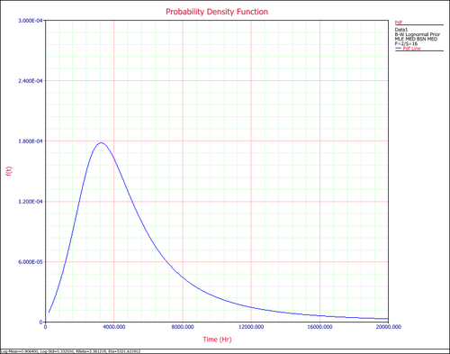
The pdf of the times-to-failure data can be plotted in Weibull++, as shown next:


