BlockSim Analytical Examples

BlockSim Analytical Example

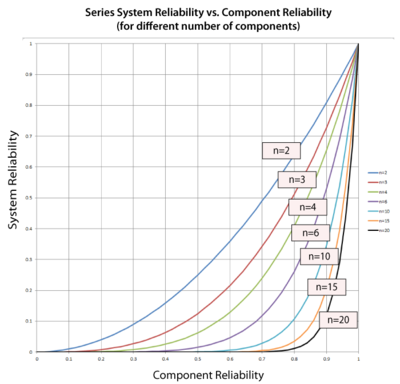
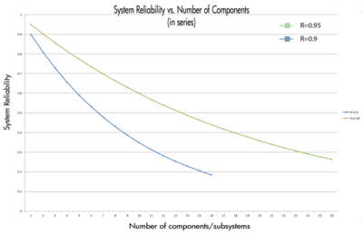
Consider a system that consists of a single component. The reliability of the component is 95%, thus the reliability of the system is 95%. What would the reliability of the system be if there were more than one component (with the same individual reliability) in series? Table 2 shows the effect on the system's reliability by adding consecutive components (with the same reliability) in series. Figure Ch4fig6 illustrates the same concept graphically for components with 90% and 95% reliability.

BlockSim Analytical Example

Consider a system consisting of three subsystems arranged reliability-wise in parallel. Subsystem 1 has a reliability of 99.5%, Subsystem 2 has a reliability of 98.7% and Subsystem 3 has a reliability of 97.3% for a mission of 100 hours. What is the overall reliability of the system for a 100-hour mission?

Solution

Since the reliabilities of the subsystems are specified for 100 hours, the reliability of the system for a 100-hour mission is: ..

BlockSim Analytical Example

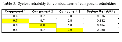
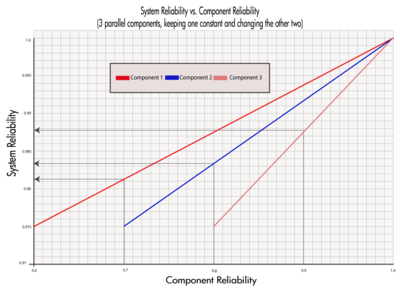
Consider three components arranged reliability-wise in parallel with .. = 60%, [math]\displaystyle{ {{R}_{2}} }[/math] = 70% and [math]\displaystyle{ {{R}_{3}} }[/math] = 80% (for a given time). The corresponding reliability for the system is [math]\displaystyle{ {{R}_{s}} }[/math] = 97.6%. In Table 3, we can examine the effect of each component's reliability on the overall system reliability. The first row of the table shows the given reliability for each component and the corresponding system reliability for these values. In the second row, the reliability of Component 1 is increased by a value of 10% while keeping the reliabilities of the other two components constant. Similarly, by increasing the reliabilities of Components 2 and 3 in the third and fourth rows by a value of 10% while keeping the reliabilities of the other components at the given values, we can observe the effect of each component's reliability on the overall system reliability. It is clear that the highest value for the system's reliability was achieved when the reliability of Component 3, which is the most reliable component, was increased. Once again, this is the opposite of what was encountered with a pure series system.

This conclusion can also be illustrated graphically, as shown in Figure 4.6.

Effect of Number of Components in Parallel

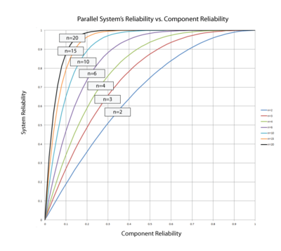
In the case of the parallel configuration, the number of components has the opposite effect of the one observed for the series configuration. For a parallel configuration, as the number of components/subsystems increases, the system's reliability increases.
Figure 4.7 illustrates that a high system reliability can be achieved with low-reliability components, provided that there are a sufficient number of components in parallel. Note that Figure Ch4fig9 is the mirror image of Figure 4.7, which presents the effect of the number of components in a series configuration.

BlockSim Analytical Example

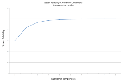
Consider a system that consists of a single component. The reliability of the component is 60%, thus the reliability of the system is 60%. What would the reliability of the system be if the system were composed of two, four or six such components in parallel?

Clearly, the reliability of a system can be improved by adding redundancy. However, it must be noted that doing so is usually costly in terms of additional components, additional weight, volume, etc.
Reliability optimization and costs are covered in detail in Chapter 6.

BlockSim Analytical Example

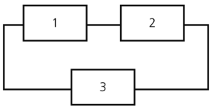
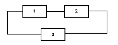
Consider a system with three components. Units 1 and 2 are connected in series and Unit 3 is connected in parallel with the first two, as shown in the next figure.

What is the reliability of the system if [math]\displaystyle{ {{R}_{1}} }[/math] = 99.5%, [math]\displaystyle{ {{R}_{2}} }[/math] = 98.7% and [math]\displaystyle{ {{R}_{3}} }[/math] = 97.3% at 100 hours?

Solution

First, the reliability of the series segment consisting of Units 1 and 2 is calculated:

[math]\displaystyle{ \begin{align} {{R}_{1,2}}= & {{R}_{1}}\cdot {{R}_{2}} \\ {{R}_{1,2}}= & 0.9950\cdot 0.9870 \\ {{R}_{1,2}}= & 0.982065\text{ or }98.2065% \end{align} }[/math]

The reliability of the overall system is then calculated by treating Units 1 and 2 as one unit with a reliability of 98.2065% connected in parallel with Unit 3. Therefore:

[math]\displaystyle{ \begin{align} {{R}_{s}}= & 1-[(1-0.982065)\cdot (1-0.973000)] \\ {{R}_{s}}= & 1-0.000484245 \\ {{R}_{s}}= & 0.999515755 \\ {{R}_{s}}= & 99.95% \end{align} }[/math]

BlockSim Analytical Example

Consider a system of six pumps of which at least four must function properly for system success. Each pump has an 85% reliability for the mission duration. What is the probability of success of the system for the same mission duration?

Solution

Using Eqn. (binomial) for [math]\displaystyle{ k=4 }[/math] and [math]\displaystyle{ n=6 }[/math] :

[math]\displaystyle{ \begin{align} {{R}_{s}}= & \underset{r=4}{\overset{6}{\mathop \sum }}\,\left( \begin{matrix} 6 \\ r \\ \end{matrix} \right){{0.85}^{r}}{{(1-0.85)}^{6-r}} \\ = & \left( \begin{matrix} 6 \\ 4 \\ \end{matrix} \right){{0.85}^{4}}{{(1-0.85)}^{2}}+\left( \begin{matrix} 6 \\ 5 \\ \end{matrix} \right){{0.85}^{5}}{{(1-0.85)}^{1}} \\ & +\left( \begin{matrix} 6 \\ 6 \\ \end{matrix} \right){{0.85}^{6}}{{(1-0.85)}^{0}} \\ = & 0.1762+0.3993+0.3771 \\ = & 95.26% \end{align} }[/math]

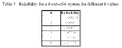
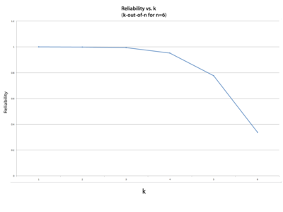
One can examine the effect of increasing the number of units required for system success while the total number of units remains constant (in this example, six units). In Figure Ch4fig12, the reliability of the [math]\displaystyle{ k }[/math] -out-of-6 configuration was plotted versus different numbers of required units.

Note that the system configuration becomes a simple parallel configuration for [math]\displaystyle{ k }[/math] = 1 and the system is a six-unit series configuration ( [math]\displaystyle{ {{(0.85)}^{6}}= }[/math] 0.377) for [math]\displaystyle{ k }[/math] = 6. [math]\displaystyle{ }[/math]

BlockSim Analytical Example

Three hard drives in a computer system are configured reliability-wise in parallel. At least two of them must function in order for the computer to work properly. Each hard drive is of the same size and speed, but they are made by different manufacturers and have different reliabilities. The reliability of [math]\displaystyle{ HD\#1 }[/math] is 0.9, [math]\displaystyle{ HD\#2 }[/math] is 0.88 and [math]\displaystyle{ HD\#3 }[/math] is 0.85, all at the same mission time.

Solution

Since at least two hard drives must be functioning at all times, only one failure is allowed. This is a 2-out-of-3 configuration.
The following operational combinations are possible for system success:

1. All 3 hard drives operate.
2. [math]\displaystyle{ HD\#1 }[/math] fails, while [math]\displaystyle{ HDs\,\#2 }[/math] and [math]\displaystyle{ \#3 }[/math] continue to operate.
3. [math]\displaystyle{ HD\#2 }[/math] fails, while [math]\displaystyle{ HDs\,\#1 }[/math] and [math]\displaystyle{ \#3 }[/math] continue to operate.
4. [math]\displaystyle{ HD\#3 }[/math] fails, while [math]\displaystyle{ HDs\,\#1 }[/math] and [math]\displaystyle{ \#2 }[/math] continue to operate.

The probability of success for the system (reliability) can now be expressed as:

[math]\displaystyle{ \begin{align} {{P}_{s}}= & {{R}_{1}}{{R}_{2}}{{R}_{3}}+(1-{{R}_{1}}){{R}_{2}}{{R}_{3}}+{{R}_{1}}(1-{{R}_{2}}){{R}_{3}} \\ & +{{R}_{1}}{{R}_{2}}(1-{{R}_{3}}) \end{align} }[/math]

This equation for the reliability of the system can be reduced to:

[math]\displaystyle{ {{R}_{s}}={{R}_{1}}{{R}_{2}}+{{R}_{2}}{{R}_{3}}+{{R}_{1}}{{R}_{3}}-2{{R}_{1}}{{R}_{2}}{{R}_{3}} }[/math]

Or:

[math]\displaystyle{ {{R}_{s}}=95.86% }[/math]

If all three hard drives had the same reliability, [math]\displaystyle{ R }[/math] , then the equation for the reliability of the system could be further reduced to:

[math]\displaystyle{ {{R}_{s}}=3{{R}^{2}}-2{{R}^{3}} }[/math]

Or, using the binomial approach:

[math]\displaystyle{ \begin{align} {{R}_{s}}= & \underset{r=2}{\overset{3}{\mathop \sum }}\,\left( \begin{matrix} 3 \\ r \\ \end{matrix} \right){{R}^{r}}{{(1-R)}^{3-r}} \\ = & \left( \begin{matrix} 3 \\ 2 \\ \end{matrix} \right){{R}^{2}}(1-R)+\left( \begin{matrix} 3 \\ 3 \\ \end{matrix} \right){{R}^{3}}{{(1-R)}^{0}} \\ = & 3\cdot {{R}^{2}}(1-R)+{{R}^{3}} \\ = & 3{{R}^{2}}-2{{R}^{3}} \end{align} }[/math]

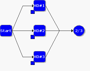
The example can be repeated using BlockSim. The following graphic demonstrates the RBD for the system.
[math]\displaystyle{ }[/math]

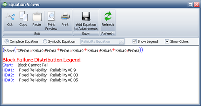
The RBD is analyzed and the system reliability equation is returned. Figure Ch4fig15 shows the equation returned by BlockSim.

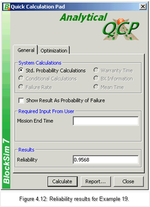
Using the Analytical Quick Calculation Pad, the reliability can be calculated to be 0.9586. Figure 4.11 shows the returned result.
Note that you are not required to enter a mission end time for this system into the Analytical QCP because all of the components are static and thus the reliability results are independent of time.

BlockSim Analytical Example

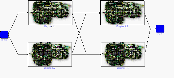
Consider the four-engine aircraft discussed previously. If we were to change the problem statement to two out of four engines are required, however no two engines on the same side may fail, then the block diagram would change to the configuration shown in Figure example10.
[math]\displaystyle{ }[/math]
Note that this is the same as having two engines in parallel on each wing and then putting the two wings in series.

Block diagram for Example 10

RBD for the consecutive k-out-of-n: F system

BlockSim Analytical Example

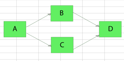
Obtain the reliability equation of the following system.

Solution

The successful paths for this system are:

[math]\displaystyle{ {{X}_{1}}=ABD\text{ and }{{X}_{2}}=ACD }[/math]

The reliability of the system is simply the probability of the union of these paths:

[math]\displaystyle{ {{R}_{s}}=P({{X}_{1}}\cup {{X}_{2}}) }[/math]

[math]\displaystyle{ \begin{align} P({{X}_{1}}\cup {{X}_{2}})= & P({{X}_{1}})+P({{X}_{2}})-P({{X}_{1}}\cap {{X}_{2}}) \\ = & P(ABD)+P(ACD)-P(ABCD) \end{align} }[/math]

Thus:

[math]\displaystyle{ {{R}_{s}}={{R}_{A}}{{R}_{B}}{{R}_{D}}+{{R}_{A}}{{R}_{C}}{{R}_{D}}-{{R}_{A}}{{R}_{B}}{{R}_{C}}{{R}_{D}} }[/math]

BlockSim Analytical Example

Obtain the reliability equation of the following system.

BlockSim Analytical Example

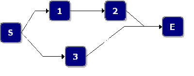
Assume starting and ending blocks that cannot fail, as shown next.

The paths for this system are:

[math]\displaystyle{ {{X}_{1}}=1,2\text{ and }{{X}_{2}}=3 }[/math]

The probability of success of the system is given by:

[math]\displaystyle{ \begin{align} P({{X}_{1}}\cup {{X}_{2}})= & P({{X}_{1}})+P({{X}_{2}})-P({{X}_{1}}\cap {{X}_{2}}) \\ = & P(1,2)+P(3)-P(1,2,3) \end{align} }[/math]

Or:

[math]\displaystyle{ {{R}_{s}}={{R}_{1}}{{R}_{2}}+{{R}_{3}}-{{R}_{1}}{{R}_{2}}{{R}_{3}} }[/math]

Starting and Ending Blocks in BlockSim

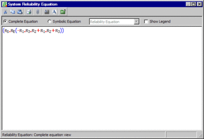
Note that BlockSim requires that all diagrams start from a single block and end on a single block. To meet this requirement for this example, we arbitrarily added a starting and an ending block, as shown in Figure Ch4fig21. These blocks can be set to a cannot fail condition, or [math]\displaystyle{ R=1 }[/math] , and thus not affect the outcome. However, when the analysis is performed in BlockSim, the returned equation will include terms for the non-failing blocks, as shown in Figure Ch4fig22 and Eqn. (8).

[math]\displaystyle{ {{R}_{system}}=({{R}_{S}}\cdot {{R}_{E}}(-{{R}_{1}}\cdot {{R}_{2}}\cdot {{R}_{3}}+{{R}_{1}}\cdot {{R}_{2}}+{{R}_{3}})) }[/math]

Note that since [math]\displaystyle{ {{R}_{S}}={{R}_{E}}=1 }[/math] , the system equation, Eqn. (eqnonfailed), can be reduced to:

[math]\displaystyle{ \begin{align} {{R}_{system}}= & (1\cdot 1(-{{R}_{1}}\cdot {{R}_{2}}\cdot {{R}_{3}}+{{R}_{1}}\cdot {{R}_{2}}+{{R}_{3}})) \\ = & -{{R}_{1}}\cdot {{R}_{2}}\cdot {{R}_{3}}+{{R}_{1}}\cdot {{R}_{2}}+{{R}_{3}} \end{align} }[/math]

This is equivalent to Eqn. (ex11s). The reason that BlockSim includes all items regardless of whether they can fail or not is because BlockSim only recomputes the equation when the system structure has changed. What this means is that the user can alter the failure characteristics of an item without altering the diagram structure. For example, a block that was originally set not to fail can be re-set to a failure distribution and thus it would need to be used in subsequent analyses.

BlockSim representation of the RBD for Example 12.

BlockSim solution to the TBD in Figure 4.16.

BlockSim Analytical Example

For this example:

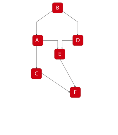
[math]\displaystyle{ a) }[/math] Determine the reliability equation of the system shown in Figure Ch4fig9 using the decomposition method.

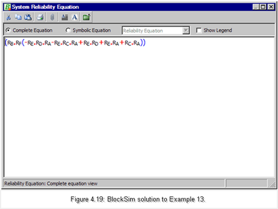
[math]\displaystyle{ b) }[/math] Determine the reliability equation of the same system using BlockSim.

Solution

To obtain the solution:

[math]\displaystyle{ a) }[/math] Choose A as the key component, then:

[math]\displaystyle{ \begin{align} {{R}_{s}}= & P(s|A)P(A)+P(s|\overline{A})P(\overline{A}) \\ P(s| A)= &{{R}_{B}}{{R}_{F}}\left[ 1-\left( 1-{{R}_{C}} \right)\left( 1-{{R}_{E}} \right) \right] \\ P(s| \overline{A})= &{{R}_{B}}{{R}_{D}}{{R}_{E}}{{R}_{F}} \\ {{R}_{s}}= & \left[ {{R}_{B}}{{R}_{F}}\left[ 1-\left( 1-{{R}_{C}} \right)\left( 1-{{R}_{E}} \right) \right] \right]{{R}_{A}}+\left[ {{R}_{B}}{{R}_{D}}{{R}_{E}}{{R}_{F}} \right](1-{{R}_{A}}) \end{align} }[/math]

[math]\displaystyle{ b) }[/math] Using BlockSim:

[math]\displaystyle{ {{R}_{s}}={{R}_{B}}\cdot {{R}_{F}}(-{{R}_{A}}\cdot {{R}_{C}}\cdot {{R}_{E}}-{{R}_{A}}\cdot {{R}_{D}}\cdot {{R}_{E}}+{{R}_{A}}\cdot {{R}_{C}}+{{R}_{A}}\cdot {{R}_{E}}+{{R}_{D}}\cdot {{R}_{E}}) }[/math]

Diagram for Example 13.

BlockSim solution to Example 13

BlockSim Analytical Example

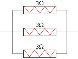
Consider the following circuit:

The equivalent resistance must always be less than [math]\displaystyle{ 1.2\Omega }[/math] .
Draw the reliability block diagram for this circuit.

Solution

First, let's consider the case where all three resistors operate:

[math]\displaystyle{ \begin{align} \frac{1}{{{r}_{eq}}}= & \frac{1}{{{r}_{1}}}+\frac{1}{{{r}_{2}}}+\frac{1}{{{r}_{3}}} \\ = & \frac{1}{3}+\frac{1}{3}+\frac{1}{3} \\ = & 1\Omega \end{align} }[/math]

Thus, when all components operate, the equivalent resistance is [math]\displaystyle{ 1\Omega }[/math] , which is less than the maximum resistance of [math]\displaystyle{ 1.2\Omega }[/math] .

Next, consider the case where one of the resistors fails open. In this case, the resistance for the resistor is infinite and the equivalent resistance is:

[math]\displaystyle{ \frac{1}{{{r}_{eq}}}=\frac{1}{\infty }+\frac{1}{3}+\frac{1}{3}=\frac{2}{3} }[/math]

Thus:

[math]\displaystyle{ {{r}_{eq}}=1.5\Omega \gt 1.2\Omega \text{ - System failed}\text{.} }[/math]

If two resistors fail open (e.g. #1 and #2), the equivalent resistance is:

[math]\displaystyle{ \frac{1}{{{r}_{eq}}}=\frac{1}{\infty }+\frac{1}{\infty }+\frac{1}{3}=\frac{1}{3} }[/math]

Thus:

[math]\displaystyle{ {{r}_{eq}}=3\Omega \gt 1.2\Omega \text{ - System failed}\text{.} }[/math]

If all three resistors fail open:

[math]\displaystyle{ {{r}_{eq}}=\infty \gt 1.2\Omega \text{ - System failed}\text{.} }[/math]

Thus, if [math]\displaystyle{ {{r}_{1}} }[/math] , [math]\displaystyle{ {{r}_{2}} }[/math] , [math]\displaystyle{ {{r}_{3}} }[/math], or any combination of the three fails, the system fails. Put another way, [math]\displaystyle{ {{r}_{1}} }[/math] and [math]\displaystyle{ {{r}_{2}} }[/math] and [math]\displaystyle{ {{r}_{3}} }[/math] must succeed in order for the system to succeed.
The RBD is:

In this example it can be seen that even though the three components were physically arranged in parallel, their reliability-wise arrangement is in series.

Example 15

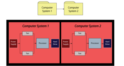
For this example, obtain the reliability equation of the system shown in Figure fig29.

Solution to Example 15

The system reliability equation is:

[math]\displaystyle{ {{R}_{System}}={{R}_{Computer1}}\cdot {{R}_{Computer2}} }[/math]

Now:

[math]\displaystyle{ \begin{align} {{R}_{Computer1}}= & ({{R}_{Power\,Supply}}\cdot {{R}_{Processor}}\cdot {{R}_{HardDrive}} \\ &\cdot(-{{R}_{Fan}}\cdot {{R}_{Fan}}+{{R}_{Fan}}+{{R}_{Fan}})) \end{align} }[/math]

Since the structures of the computer systems are the same, [math]\displaystyle{ {{R}_{Computer1}}={{R}_{Computer2}} }[/math] , then substituting Eqn. (excomp2a) into Eqn. (excomp) yields:

[math]\displaystyle{ \begin{align} {{R}_{System}}= & ({{R}_{Power\,Supply}}\cdot {{R}_{Processor}}) \\ & \cdot {{R}_{HardDrive}}(-R_{Fan}^{2}+2{{R}_{Fan}}){{)}^{2}} \end{align} }[/math]

When using BlockSim to compute the equation, the software will return Eqn. (excomp) for the system and Eqn. (excomp2a) for the subdiagram. Even though BlockSim will make these substitutions internally when performing calculations, it does show them in the System Reliability Equation window.

Illustration of subdiagrams.

Example 16

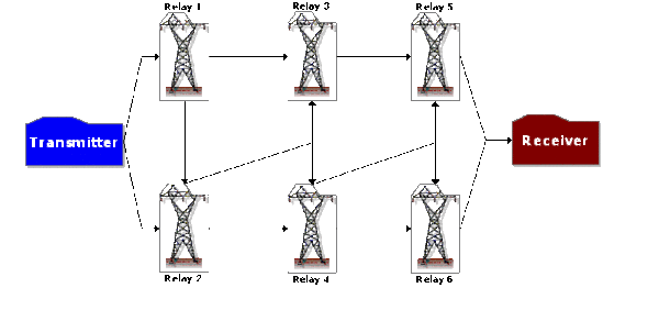
In the diagram shown in Figure Fig32, electricity can flow in both directions. Successful system operation requires at least one output (O1, O2 or O3) to be working.

Create a block diagram for this system.

Solution to Example 16

The bidirectionality of this system can be modeled using mirrored blocks. The diagram is shown in Figure fig33a.

Blocks 5A, 7A and 1A are duplicates (or mirrored blocks) of 5, 7 and 1 respectively.

Example 18

Assume that a system has six failure modes: A, B, C, D, E and F. Furthermore, assume that failure of the entire system will occur if:

• Mode B, C or F occurs.

• Modes A and E, A and D or E and D occur.

Draw the block diagram and obtain the reliability equation.

Solution to Example 18

The diagram is shown in Figure fig35

The reliability equation, as obtained from BlockSim is:

[math]\displaystyle{ \begin{align} {{R}_{System}}= & (-2{{R}_{A}}\cdot {{R}_{B}}\cdot {{R}_{C}}\cdot {{R}_{D}}\cdot {{R}_{2/3}}\cdot {{R}_{E}}\cdot {{R}_{F}} \\ & +{{R}_{A}}\cdot {{R}_{B}}\cdot {{R}_{C}}\cdot {{R}_{D}}\cdot {{R}_{2/3}}\cdot {{R}_{F}} \\ & +{{R}_{A}}\cdot {{R}_{B}}\cdot {{R}_{C}}\cdot {{R}_{2/3}}\cdot {{R}_{E}}\cdot {{R}_{F}} \\ & +{{R}_{B}}\cdot {{R}_{C}}\cdot {{R}_{D}}\cdot {{R}_{2/3}}\cdot {{R}_{E}}\cdot {{R}_{F}}) \end{align} }[/math]

The BlockSim equation includes the node reliability term [math]\displaystyle{ {{R}_{2/3}}, }[/math] which cannot fail, or [math]\displaystyle{ {{R}_{2/3}}=1 }[/math] . This can be removed, yielding:

[math]\displaystyle{ \begin{align} {{R}_{System}}= & (-2{{R}_{A}}\cdot {{R}_{B}}\cdot {{R}_{C}}\cdot {{R}_{D}}\cdot {{R}_{E}}\cdot {{R}_{F}} \\ & +{{R}_{A}}\cdot {{R}_{B}}\cdot {{R}_{C}}\cdot {{R}_{D}}\cdot {{R}_{F}} \\ & +{{R}_{A}}\cdot {{R}_{B}}\cdot {{R}_{C}}\cdot {{R}_{E}}\cdot {{R}_{F}} \\ & +{{R}_{B}}\cdot {{R}_{C}}\cdot {{R}_{D}}\cdot {{R}_{E}}\cdot {{R}_{F}}) \end{align} }[/math]