Change of Slope Analysis Example
New format available! This reference is now available in a new format that offers faster page load, improved display for calculations and images and more targeted search.
As of January 2024, this Reliawiki page will not continue to be updated. Please update all links and bookmarks to the latest references at RGA examples and RGA reference examples.
This example appears in the article Change of Slope Analysis.
The following table gives the failure times obtained from a reliability growth test of a newly designed system. The test has a duration of 660 hours.
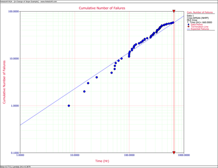
First, apply a single Crow-AMSAA (NHPP) model to all of the data. The following plot shows the expected failures obtained from the model (the line) along with the observed failures (the points).
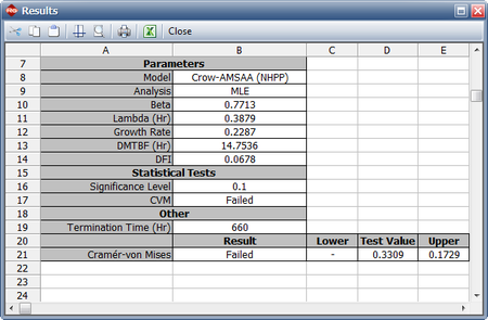
The plot shows that the model does not seem to accurately track the data. This is confirmed by performing the Cramér-von Mises goodness-of-fit test, which checks the hypothesis that the data follows a non-homogeneous Poisson process with a power law failure intensity. The model fails the goodness-of-fit test because the test statistic (0.3309) is higher than the critical value (0.1729) at the 0.1 significance level. The next figure shows a customized report that displays both the calculated parameters and the statistical test results.
Through further investigation, it is discovered that a significant design change occurred at 400 hours of test time. It is suspected that this modification is responsible for the change in the failure behavior.
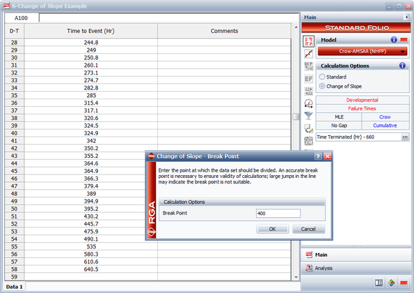
In RGA, you have the option to perform a standard Crow-AMSAA (NHPP) analysis, or perform a Change of Slope analysis where you specify a specific breakpoint, as shown in the following figure. RGA actually creates a grouped data set where the data in Segment 1 is included and defined by a single interval to calculate the Segment 2 parameters. However, these results are equivalent to the parameters estimated using the equations presented here.
Therefore, the Change of Slope methodology is applied to break the data into two segments for analysis. The first segment is set from 0 to 400 hours and the second segment is from 401 to 660 hours (which is the end time of the test). The Crow-AMSAA (NHPP) parameters for the first segment (0-400 hours) are:
- [math]\displaystyle{ \widehat{{{\lambda }_{1}}}=\frac{{{n}_{1}}}{T_{1}^{{{\beta }_{1}}}}=\frac{50}{{{400}^{1.0359}}}=0.1008\,\! }[/math]
and
- [math]\displaystyle{ {{\widehat{\beta }}_{1}}=\frac{{{n}_{1}}}{\underset{i=1}{\overset{{{n}_{1}}}{\mathop{\sum }}}\,\ln \tfrac{{{T}_{1}}}{{{t}_{i}}}}=\frac{50}{\underset{i=1}{\overset{50}{\mathop{\sum }}}\,\ln \tfrac{400}{{{t}_{i}}}}=1.0359\,\! }[/math]
The Crow-AMSAA (NHPP) parameters for the second segment (401-660 hours) are:
- [math]\displaystyle{ \widehat{{{\lambda }_{2}}}=\frac{{{n}}}{T_{2}^{{{\beta }_{2}}}}=\frac{58}{{{660}^{0.2971}}}=8.4304\,\! }[/math]
- [math]\displaystyle{ {{\widehat{\beta }}_{2}}=\frac{{{n}_{2}}}{{{n}_{1}}\ln \tfrac{{{T}_{2}}}{{{T}_{1}}}+\underset{i={{n}_{1}}+1}{\overset{n}{\mathop{\sum }}}\,\ln \tfrac{{{T}_{2}}}{{{t}_{i}}}}=\frac{8}{50\ln \tfrac{660}{400}+\underset{i=51}{\overset{58}{\mathop{\sum }}}\,\ln \tfrac{660}{{{T}_{i}}}}=0.2971\,\! }[/math]
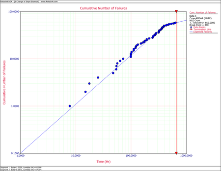
The following figure shows a plot of the two-segment analysis along with the observed data. It is obvious that the Change of Slope method tracks the data more accurately.
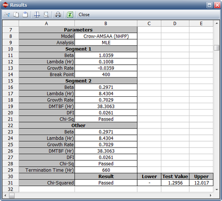
This can also be verified by performing a chi-squared goodness-of-fit test. The chi-squared statistic is 1.2956, which is lower than the critical value of 12.017 at the 0.1 significance level; therefore, the analysis passes the test. The next figure shows a customized report that displays both the calculated parameters and the statistical test results.
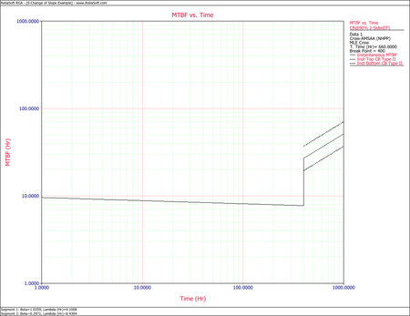
When you have a model that fits the data, it can be used to make accurate predictions and calculations. Metrics such as the demonstrated MTBF at the end of the test or the expected number of failures at later times can be calculated. For example, the following plot shows the instantaneous MTBF vs. time, together with the two-sided 90% confidence bounds. Note that confidence bounds are available for the second segment only. For times up to 400 hours, the parameters of the first segment were used to calculate the MTBF, while the parameters of the second segment were used for times after 400 hours. Also note that the number of failures at the end of segment 1 is not assumed to be equal to the number of failures at the start of segment 2. This can result in a visible jump in the plot, as in this example.
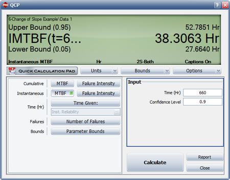
The next figure shows the use of the Quick Calculation Pad (QCP) in the RGA software to calculate the Demonstrated MTBF at the end of the test (instantaneous MTBF at time = 660), together with the two-sided 90% confidence bounds. All the calculations were based on the parameters of the second segment.

