Crow-AMSAA (NHPP)

Dr. Larry H. Crow [17] noted that the Duane Model could be stochastically represented as a Weibull process, allowing for statistical procedures to be used in the application of this model in reliability growth. This statistical extension became what is known as the Crow-AMSAA (NHPP) model. This method was first developed at the U.S. Army Materiel Systems Analysis Activity (AMSAA). It is frequently used on systems when usage is measured on a continuous scale. It can also be applied for the analysis of one shot items when there is high reliability and a large number of trials.

Test programs are generally conducted on a phase by phase basis. The Crow-AMSAA model is designed for tracking the reliability within a test phase and not across test phases. A development testing program may consist of several separate test phases. If corrective actions are introduced during a particular test phase, then this type of testing and the associated data are appropriate for analysis by the Crow-AMSAA model. The model analyzes the reliability growth progress within each test phase and can aid in determining the following:

• Reliability of the configuration currently on test
• Reliability of the configuration on test at the end of the test phase
• Expected reliability if the test time for the phase is extended
• Growth rate
• Confidence intervals
• Applicable goodness-of-fit tests

Background

The reliability growth pattern for the Crow-AMSAA model is exactly the same pattern as for the Duane postulate, that is, the cumulative number of failures is linear when plotted on ln-ln scale. Unlike the Duane postulate, the Crow-AMSAA model is statistically based. Under the Duane postulate, the failure rate is linear on ln-ln scale. However, for the Crow-AMSAA model statistical structure, the failure intensity of the underlying non-homogeneous Poisson process (NHPP) is linear when plotted on ln-ln scale.

Let [math]\displaystyle{ N(t)\,\! }[/math] be the cumulative number of failures observed in cumulative test time [math]\displaystyle{ t\,\! }[/math], and let [math]\displaystyle{ \rho (t)\,\! }[/math] be the failure intensity for the Crow-AMSAA model. Under the NHPP model, [math]\displaystyle{ \rho (t)\Delta t\,\! }[/math] is approximately the probably of a failure occurring over the interval [math]\displaystyle{ [t,t+\Delta t]\,\! }[/math] for small [math]\displaystyle{ \Delta t\,\! }[/math]. In addition, the expected number of failures experienced over the test interval [math]\displaystyle{ [0,T]\,\! }[/math] under the Crow-AMSAA model is given by:

[math]\displaystyle{ E[N(T)]=\int_{0}^{T}\rho (t)dt\,\! }[/math]

The Crow-AMSAA model assumes that [math]\displaystyle{ \rho (T)\,\! }[/math] may be approximated by the Weibull failure rate function:

[math]\displaystyle{ \rho (T)=\frac{\beta }{{{\eta }^{\beta }}}{{T}^{\beta -1}}\,\! }[/math]

Therefore, if [math]\displaystyle{ \lambda =\tfrac{1}{{{\eta }^{\beta }}},\,\! }[/math] the intensity function, [math]\displaystyle{ \rho (T),\,\! }[/math] or the instantaneous failure intensity, [math]\displaystyle{ {{\lambda }_{i}}(T)\,\! }[/math], is defined as:

[math]\displaystyle{ {{\lambda }_{i}}(T)=\lambda \beta {{T}^{\beta -1}},\text{with }T\gt 0,\text{ }\lambda \gt 0\text{ and }\beta \gt 0\,\! }[/math]

In the special case of exponential failure times, there is no growth and the failure intensity, [math]\displaystyle{ \rho (t)\,\! }[/math], is equal to [math]\displaystyle{ \lambda \,\! }[/math]. In this case, the expected number of failures is given by:

[math]\displaystyle{ \begin{align} E[N(T)]= & \int_{0}^{T}\rho (t)dt \\ = & \lambda T \end{align}\,\! }[/math]

In order for the plot to be linear when plotted on ln-ln scale under the general reliability growth case, the following must hold true where the expected number of failures is equal to:

[math]\displaystyle{ \begin{align} E[N(T)]= & \int_{0}^{T}\rho (t)dt \\ = & \lambda {{T}^{\beta }} \end{align}\,\! }[/math]

To put a statistical structure on the reliability growth process, consider again the special case of no growth. In this case the number of failures, [math]\displaystyle{ N(T),\,\! }[/math] experienced during the testing over [math]\displaystyle{ [0,T]\,\! }[/math] is random. The expected number of failures, [math]\displaystyle{ N(T),\,\! }[/math] is said to follow the homogeneous (constant) Poisson process with mean [math]\displaystyle{ \lambda T\,\! }[/math] and is given by:

[math]\displaystyle{ \underset{}{\overset{}{\mathop{\Pr }}}\,[N(T)=n]=\frac{{{(\lambda T)}^{n}}{{e}^{-\lambda T}}}{n!};\text{ }n=0,1,2,\ldots \,\! }[/math]

The Crow-AMSAA model generalizes this no growth case to allow for reliability growth due to corrective actions. This generalization keeps the Poisson distribution for the number of failures but allows for the expected number of failures, [math]\displaystyle{ E[N(T)],\,\! }[/math] to be linear when plotted on ln-ln scale. The Crow-AMSAA model lets [math]\displaystyle{ E[N(T)]=\lambda {{T}^{\beta }}\,\! }[/math]. The probability that the number of failures, [math]\displaystyle{ N(T),\,\! }[/math] will be equal to [math]\displaystyle{ n\,\! }[/math] under growth is then given by the Poisson distribution:

[math]\displaystyle{ \underset{}{\overset{}{\mathop{\Pr }}}\,[N(T)=n]=\frac{{{(\lambda {{T}^{\beta }})}^{n}}{{e}^{-\lambda {{T}^{\beta }}}}}{n!};\text{ }n=0,1,2,\ldots \,\! }[/math]

This is the general growth situation, and the number of failures, [math]\displaystyle{ N(T)\,\! }[/math], follows a non-homogeneous Poisson process. The exponential, "no growth" homogeneous Poisson process is a special case of the non-homogeneous Crow-AMSAA model. This is reflected in the Crow-AMSAA model parameter where [math]\displaystyle{ \beta =1\,\! }[/math]. The cumulative failure rate, [math]\displaystyle{ {{\lambda }_{c}}\,\! }[/math], is:

[math]\displaystyle{ \begin{align} {{\lambda }_{c}}=\lambda {{T}^{\beta -1}} \end{align}\,\! }[/math]

The cumulative [math]\displaystyle{ MTB{{F}_{c}}\,\! }[/math] is:

[math]\displaystyle{ MTB{{F}_{c}}=\frac{1}{\lambda }{{T}^{1-\beta }}\,\! }[/math]

As mentioned above, the local pattern for reliability growth within a test phase is the same as the growth pattern observed by Duane. The Duane [math]\displaystyle{ MTB{{F}_{c}}\,\! }[/math] is equal to:

[math]\displaystyle{ MTB{{F}_{{{c}_{DUANE}}}}=b{{T}^{\alpha }}\,\! }[/math]

And the Duane cumulative failure rate, [math]\displaystyle{ {{\lambda }_{c}}\,\! }[/math], is:

[math]\displaystyle{ {{\lambda }_{{{c}_{DUANE}}}}=\frac{1}{b}{{T}^{-\alpha }}\,\! }[/math]

Thus a relationship between Crow-AMSAA parameters and Duane parameters can be developed, such that:

[math]\displaystyle{ \begin{align} {{b}_{DUANE}}= & \frac{1}{{{\lambda }_{AMSAA}}} \\ {{\alpha }_{DUANE}}= & 1-{{\beta }_{AMSAA}} \end{align}\,\! }[/math]

Note that these relationships are not absolute. They change according to how the parameters (slopes, intercepts, etc.) are defined when the analysis of the data is performed. For the exponential case, [math]\displaystyle{ \beta =1\,\! }[/math], then [math]\displaystyle{ {{\lambda }_{i}}(T)=\lambda \,\! }[/math], a constant. For [math]\displaystyle{ \beta \gt 1\,\! }[/math], [math]\displaystyle{ {{\lambda }_{i}}(T)\,\! }[/math] is increasing. This indicates a deterioration in system reliability. For [math]\displaystyle{ \beta \lt 1\,\! }[/math], [math]\displaystyle{ {{\lambda }_{i}}(T)\,\! }[/math] is decreasing. This is indicative of reliability growth. Note that the model assumes a Poisson process with the Weibull intensity function, not the Weibull distribution. Therefore, statistical procedures for the Weibull distribution do not apply for this model. The parameter [math]\displaystyle{ \lambda \,\! }[/math] is called a scale parameter because it depends upon the unit of measurement chosen for [math]\displaystyle{ T\,\! }[/math], while [math]\displaystyle{ \beta \,\! }[/math] is the shape parameter that characterizes the shape of the graph of the intensity function.

The total number of failures, [math]\displaystyle{ N(T)\,\! }[/math], is a random variable with Poisson distribution. Therefore, the probability that exactly [math]\displaystyle{ n\,\! }[/math] failures occur by time [math]\displaystyle{ T\,\! }[/math] is:

[math]\displaystyle{ P[N(T)=n]=\frac{{{[\theta (T)]}^{n}}{{e}^{-\theta (T)}}}{n!}\,\! }[/math]

The number of failures occurring in the interval from [math]\displaystyle{ {{T}_{1}}\,\! }[/math] to [math]\displaystyle{ {{T}_{2}}\,\! }[/math] is a random variable having a Poisson distribution with mean:

[math]\displaystyle{ \theta ({{T}_{2}})-\theta ({{T}_{1}})=\lambda (T_{2}^{\beta }-T_{1}^{\beta })\,\! }[/math]

The number of failures in any interval is statistically independent of the number of failures in any interval that does not overlap the first interval. At time [math]\displaystyle{ {{T}_{0}}\,\! }[/math], the failure intensity is [math]\displaystyle{ {{\lambda }_{i}}({{T}_{0}})=\lambda \beta T_{0}^{\beta -1}\,\! }[/math]. If improvements are not made to the system after time [math]\displaystyle{ {{T}_{0}}\,\! }[/math], it is assumed that failures would continue to occur at the constant rate [math]\displaystyle{ {{\lambda }_{i}}({{T}_{0}})=\lambda \beta T_{0}^{\beta -1}\,\! }[/math]. Future failures would then follow an exponential distribution with mean [math]\displaystyle{ m({{T}_{0}})=\tfrac{1}{\lambda \beta T_{0}^{\beta -1}}\,\! }[/math]. The instantaneous MTBF of the system at time [math]\displaystyle{ T\,\! }[/math] is:

[math]\displaystyle{ m(T)=\frac{1}{\lambda \beta {{T}^{\beta -1}}}\,\! }[/math]

Note About Applicability

The Duane and Crow-AMSAA models are the most frequently used reliability growth models. Their relationship comes from the fact that both make use of the underlying observed linear relationship between the logarithm of cumulative MTBF and cumulative test time. However, the Duane model does not provide a capability to test whether the change in MTBF observed over time is significantly different from what might be seen due to random error between phases. The Crow-AMSAA model allows for such assessments. Also, the Crow-AMSAA allows for development of hypothesis testing procedures to determine growth presence in the data (where [math]\displaystyle{ \beta \lt 1\,\! }[/math] indicates that there is growth in MTBF, [math]\displaystyle{ \beta =1\,\! }[/math] indicates a constant MTBF and [math]\displaystyle{ \beta \gt 1\,\! }[/math] indicates a decreasing MTBF). Additionally, the Crow-AMSAA model views the process of reliability growth as probabilistic, while the Duane model views the process as deterministic.

Parameter Estimation

Maximum Likelihood Estimators

The probability density function (pdf) of the [math]\displaystyle{ {{i}^{th}}\,\! }[/math] event given that the [math]\displaystyle{ {{(i-1)}^{th}}\,\! }[/math] event occurred at [math]\displaystyle{ {{T}_{i-1}}\,\! }[/math] is:

[math]\displaystyle{ f({{T}_{i}}|{{T}_{i-1}})=\frac{\beta }{\eta }{{\left( \frac{{{T}_{i}}}{\eta } \right)}^{\beta -1}}\cdot {{e}^{-\tfrac{1}{{{\eta }^{\beta }}}\left( T_{i}^{\beta }-T_{i-1}^{\beta } \right)}}\,\! }[/math]

The likelihood function is:

[math]\displaystyle{ L={{\lambda }^{n}}{{\beta }^{n}}{{e}^{-\lambda {{T}^{*\beta }}}}\underset{i=1}{\overset{n}{\mathop \prod }}\,T_{i}^{\beta -1}\,\! }[/math]

where [math]\displaystyle{ {{T}^{*}}\,\! }[/math] is the termination time and is given by:

[math]\displaystyle{ {{T}^{*}}=\left\{ \begin{matrix} {{T}_{n}}\text{ if the test is failure terminated} \\ T\gt {{T}_{n}}\text{ if the test is time terminated} \\ \end{matrix} \right\}\,\! }[/math]

Taking the natural log on both sides:

[math]\displaystyle{ \Lambda =n\ln \lambda +n\ln \beta -\lambda {{T}^{*\beta }}+(\beta -1)\underset{i=1}{\overset{n}{\mathop \sum }}\,\ln {{T}_{i}}\,\! }[/math]

And differentiating with respect to [math]\displaystyle{ \lambda \,\! }[/math] yields:

[math]\displaystyle{ \frac{\partial \Lambda }{\partial \lambda }=\frac{n}{\lambda }-{{T}^{*\beta }}\,\! }[/math]

Set equal to zero and solve for [math]\displaystyle{ \lambda \,\! }[/math] :

[math]\displaystyle{ \widehat{\lambda }=\frac{n}{{{T}^{*\beta }}}\,\! }[/math]

Now differentiate with respect to [math]\displaystyle{ \beta \,\! }[/math] :

[math]\displaystyle{ \frac{\partial \Lambda }{\partial \beta }=\frac{n}{\beta }-\lambda {{T}^{*\beta }}\ln {{T}^{*}}+\underset{i=1}{\overset{n}{\mathop \sum }}\,\ln {{T}_{i}}\,\! }[/math]

Set equal to zero and solve for [math]\displaystyle{ \beta \,\! }[/math] :

[math]\displaystyle{ \widehat{\beta }=\frac{n}{n\ln {{T}^{*}}-\underset{i=1}{\overset{n}{\mathop{\sum }}}\,\ln {{T}_{i}}}\,\! }[/math]

Biasing and Unbiasing of Beta

The equation above returns the biased estimate of [math]\displaystyle{ \beta \,\! }[/math]. The unbiased estimate of [math]\displaystyle{ \beta \,\! }[/math] can be calculated by using the following relationships. For time terminated data (meaning that the test ends after a specified number of failures):

[math]\displaystyle{ \bar{\beta }=\frac{N-1}{N}\hat{\beta }\,\! }[/math]

For failure terminated data (meaning that the test ends after a specified test time):

[math]\displaystyle{ \bar{\beta }=\frac{N-2}{N}\hat{\beta }\,\! }[/math]

Crow-AMSAA Model Example

A prototype of a system was tested with design changes incorporated during the test. The following table presents the data collected over the entire test. Find the Crow-AMSAA parameters and the intensity function using maximum likelihood estimators.

Developmental Test Data

Row	Time to Event (hr)	[math]\displaystyle{ ln{(T)}\,\! }[/math]
1	2.7	0.99325
2	10.3	2.33214
3	12.5	2.52573
4	30.6	3.42100
5	57.0	4.04305
6	61.3	4.11578
7	80.0	4.38203
8	109.5	4.69592
9	125.0	4.82831
10	128.6	4.85671
11	143.8	4.96842
12	167.9	5.12337
13	229.2	5.43459
14	296.7	5.69272
15	320.6	5.77019
16	328.2	5.79362
17	366.2	5.90318
18	396.7	5.98318
19	421.1	6.04287
20	438.2	6.08268
21	501.2	6.21701
22	620.0	6.42972

Solution

For the failure terminated test, [math]\displaystyle{ {\beta}\,\! }[/math] is:

[math]\displaystyle{ \begin{align} \widehat{\beta }&=\frac{n}{n\ln {{T}^{*}}-\underset{i=1}{\overset{n}{\mathop{\sum }}}\,\ln {{T}_{i}}} \\ &=\frac{22}{22\ln 620-\underset{i=1}{\overset{22}{\mathop{\sum }}}\,\ln {{T}_{i}}} \\ \end{align}\,\! }[/math]

where:

[math]\displaystyle{ \underset{i=1}{\overset{22}{\mathop \sum }}\,\ln {{T}_{i}}=105.6355\,\! }[/math]

Then:

[math]\displaystyle{ \widehat{\beta }=\frac{22}{22\ln 620-105.6355}=0.6142\,\! }[/math]

And for [math]\displaystyle{ {\lambda}\,\! }[/math] :

[math]\displaystyle{ \begin{align} \widehat{\lambda }&=\frac{n}{{{T}^{*\beta }}} \\ & =\frac{22}{{{620}^{0.6142}}}=0.4239 \\ \end{align}\,\! }[/math]

Therefore, [math]\displaystyle{ {{\lambda }_{i}}(T)\,\! }[/math] becomes:

[math]\displaystyle{ \begin{align} {{\widehat{\lambda }}_{i}}(T)= & 0.4239\cdot 0.6142\cdot {{620}^{-0.3858}} \\ = & 0.0217906\frac{\text{failures}}{\text{hr}} \end{align}\,\! }[/math]

The next figure shows the plot of the failure rate. If no further changes are made, the estimated MTBF is [math]\displaystyle{ \tfrac{1}{0.0217906}\,\! }[/math] or 46 hours.

Confidence Bounds

The RGA software provides two methods to estimate the confidence bounds for the Crow Extended model when applied to developmental testing data. The Fisher Matrix approach is based on the Fisher Information Matrix and is commonly employed in the reliability field. The Crow bounds were developed by Dr. Larry Crow. See the Crow-AMSAA Confidence Bounds chapter for details on how the confidence bounds are calculated.

Confidence Bounds Example

Example - Confidence Bounds on Failure Intensity

Using the values of [math]\displaystyle{ \hat{\beta }\,\! }[/math] and [math]\displaystyle{ \hat{\lambda }\,\! }[/math] estimated in the example given above, calculate the 90% 2-sided confidence bounds on the cumulative and instantaneous failure intensity.

Solution

Fisher Matrix Bounds

The partial derivatives for the Fisher Matrix confidence bounds are:

[math]\displaystyle{ \begin{align} \frac{{{\partial }^{2}}\Lambda }{\partial {{\lambda }^{2}}} = & -\frac{22}{{{0.4239}^{2}}}=-122.43 \\ \frac{{{\partial }^{2}}\Lambda }{\partial {{\beta }^{2}}} = & -\frac{22}{{{0.6142}^{2}}}-0.4239\cdot {{620}^{0.6142}}{{(\ln 620)}^{2}}=-967.68 \\ \frac{{{\partial }^{2}}\Lambda }{\partial \lambda \partial \beta } = & -{{620}^{0.6142}}\ln 620=-333.64 \end{align}\,\! }[/math]

The Fisher Matrix then becomes:

[math]\displaystyle{ \begin{align} \begin{bmatrix}122.43 & 333.64\\ 333.64 & 967.68\end{bmatrix}^{-1} & = \begin{bmatrix}Var(\hat{\lambda}) & Cov(\hat{\beta},\hat{\lambda})\\ Cov(\hat{\beta},\hat{\lambda}) & Var(\hat{\beta})\end{bmatrix} \\ & = \begin{bmatrix} 0.13519969 & -0.046614609\\ -0.046614609 & 0.017105343 \end{bmatrix} \end{align}\,\! }[/math]

For [math]\displaystyle{ T=620\,\! }[/math] hours, the partial derivatives of the cumulative and instantaneous failure intensities are:

[math]\displaystyle{ \begin{align} \frac{\partial {{\lambda }_{c}}(T)}{\partial \beta }= & \hat{\lambda }{{T}^{\hat{\beta }-1}}\ln (T) \\ = & 0.4239\cdot {{620}^{-0.3858}}\ln 620 \\ = & 0.22811336 \\ \frac{\partial {{\lambda }_{c}}(T)}{\partial \lambda }= & {{T}^{\hat{\beta }-1}} \\ = & {{620}^{-0.3858}} \\ = & 0.083694185 \end{align}\,\! }[/math]

[math]\displaystyle{ \begin{align} \frac{\partial {{\lambda }_{i}}(T)}{\partial \beta }= & \hat{\lambda }{{T}^{\hat{\beta }-1}}+\hat{\lambda }\hat{\beta }{{T}^{\hat{\beta }-1}}\ln T \\ = & 0.4239\cdot {{620}^{-0.3858}}+0.4239\cdot 0.6142\cdot {{620}^{-0.3858}}\ln 620 \\ = & 0.17558519 \end{align}\,\! }[/math]

[math]\displaystyle{ \begin{align} \frac{\partial {{\lambda }_{i}}(T)}{\partial \lambda }= & \hat{\beta }{{T}^{\hat{\beta }-1}} \\ = & 0.6142\cdot {{620}^{-0.3858}} \\ = & 0.051404969 \end{align}\,\! }[/math]

Therefore, the variances become:

[math]\displaystyle{ \begin{align} Var(\hat{\lambda_{c}}(T)) & = 0.22811336^{2}\cdot 0.017105343\ + 0.083694185^{2} \cdot 0.13519969\ -2\cdot 0.22811336\cdot 0.083694185\cdot 0.046614609 \\ & = 0.00005721408 \\ Var(\hat{\lambda_{i}}(T)) & = 0.17558519^{2}\cdot 0.01715343\ + 0.051404969^{2}\cdot 0.13519969\ -2\cdot 0.17558519\cdot 0.051404969\cdot 0.046614609 \\ &= 0.0000431393 \end{align}\,\! }[/math]

The cumulative and instantaneous failure intensities at [math]\displaystyle{ T=620\,\! }[/math] hours are:

[math]\displaystyle{ \begin{align} {{\lambda }_{c}}(T)= & 0.03548 \\ {{\lambda }_{i}}(T)= & 0.02179 \end{align}\,\! }[/math]

So, at the 90% confidence level and for [math]\displaystyle{ T=620\,\! }[/math] hours, the Fisher Matrix confidence bounds for the cumulative failure intensity are:

[math]\displaystyle{ \begin{align} {{[{{\lambda }_{c}}(T)]}_{L}}= & 0.02499 \\ {{[{{\lambda }_{c}}(T)]}_{U}}= & 0.05039 \end{align}\,\! }[/math]

The confidence bounds for the instantaneous failure intensity are:

[math]\displaystyle{ \begin{align} {{[{{\lambda }_{i}}(T)]}_{L}}= & 0.01327 \\ {{[{{\lambda }_{i}}(T)]}_{U}}= & 0.03579 \end{align}\,\! }[/math]

The following figures display plots of the Fisher Matrix confidence bounds for the cumulative and instantaneous failure intensity, respectively.

Crow Bounds

Given that the data is failure terminated, the Crow confidence bounds for the cumulative failure intensity at the 90% confidence level and for [math]\displaystyle{ T=620\,\! }[/math] hours are:

[math]\displaystyle{ \begin{align} {{[{{\lambda }_{c}}(T)]}_{L}} = & \frac{\chi _{\tfrac{\alpha }{2},2N}^{2}}{2\cdot t} \\ = & \frac{29.787476}{2*620} \\ = & 0.02402 \\ {{[{{\lambda }_{c}}(T)]}_{U}} = & \frac{\chi _{1-\tfrac{\alpha }{2},2N}^{2}}{2\cdot t} \\ = & \frac{60.48089}{2*620} \\ = & 0.048775 \end{align}\,\! }[/math]

The Crow confidence bounds for the instantaneous failure intensity at the 90% confidence level and for [math]\displaystyle{ T=620\,\! }[/math] hours are calculated by first estimating the bounds on the instantaneous MTBF. Once these are calculated, take the inverse as shown below. Details on the confidence bounds for instantaneous MTBF are presented here.

[math]\displaystyle{ \begin{align} {{[{{\lambda }_{i}}(t)]}_{L}} = & \frac{1}{{{[MTB{{F}_{i}}]}_{U}}} \\ = & \frac{1}{MTB{{F}_{i}}\cdot U} \\ = & 0.01179 \end{align}\,\! }[/math]

[math]\displaystyle{ \begin{align} {{[{{\lambda }_{i}}(t)]}_{U}}= & \frac{1}{{{[MTB{{F}_{i}}]}_{L}}} \\ = & \frac{1}{MTB{{F}_{i}}\cdot L} \\ = & 0.03253 \end{align}\,\! }[/math]

The following figures display plots of the Crow confidence bounds for the cumulative and instantaneous failure intensity, respectively.

Example - Confidence Bounds on MTBF

Calculate the confidence bounds on the cumulative and instantaneous MTBF for the data from the example given above.

Solution

Fisher Matrix Bounds

From the previous example:

[math]\displaystyle{ \begin{align} Var(\hat{\lambda }) = & 0.13519969 \\ Var(\hat{\beta }) = & 0.017105343 \\ Cov(\hat{\beta },\hat{\lambda }) = & -0.046614609 \end{align}\,\! }[/math]

And for [math]\displaystyle{ T=620\,\! }[/math] hours, the partial derivatives of the cumulative and instantaneous MTBF are:

[math]\displaystyle{ \begin{align} \frac{\partial {{m}_{c}}(T)}{\partial \beta }= & -\frac{1}{\hat{\lambda }}{{T}^{1-\hat{\beta }}}\ln T \\ = & -\frac{1}{0.4239}{{620}^{0.3858}}\ln 620 \\ = & -181.23135 \\ \frac{\partial {{m}_{c}}(T)}{\partial \lambda } = & -\frac{1}{{{\hat{\lambda }}^{2}}}{{T}^{1-\hat{\beta }}} \\ = & -\frac{1}{{{0.4239}^{2}}}{{620}^{0.3858}} \\ = & -66.493299 \\ \frac{\partial {{m}_{i}}(T)}{\partial \beta } = & -\frac{1}{\hat{\lambda }{{\hat{\beta }}^{2}}}{{T}^{1-\beta }}-\frac{1}{\hat{\lambda }\hat{\beta }}{{T}^{1-\hat{\beta }}}\ln T \\ = & -\frac{1}{0.4239\cdot {{0.6142}^{2}}}{{620}^{0.3858}}-\frac{1}{0.4239\cdot 0.6142}{{620}^{0.3858}}\ln 620 \\ = & -369.78634 \\ \frac{\partial {{m}_{i}}(T)}{\partial \lambda } = & -\frac{1}{{{\hat{\lambda }}^{2}}\hat{\beta }}{{T}^{1-\hat{\beta }}} \\ = & -\frac{1}{{{0.4239}^{2}}\cdot 0.6142}\cdot {{620}^{0.3858}} \\ = & -108.26001 \end{align}\,\! }[/math]

Therefore, the variances become:

[math]\displaystyle{ \begin{align} Var({{\hat{m}}_{c}}(T)) = & {{\left( -181.23135 \right)}^{2}}\cdot 0.017105343+{{\left( -66.493299 \right)}^{2}}\cdot 0.13519969 \\ & -2\cdot \left( -181.23135 \right)\cdot \left( -66.493299 \right)\cdot 0.046614609 \\ = & 36.113376 \end{align}\,\! }[/math]

[math]\displaystyle{ \begin{align} Var({{\hat{m}}_{i}}(T)) = & {{\left( -369.78634 \right)}^{2}}\cdot 0.017105343+{{\left( -108.26001 \right)}^{2}}\cdot 0.13519969 \\ & -2\cdot \left( -369.78634 \right)\cdot \left( -108.26001 \right)\cdot 0.046614609 \\ = & 191.33709 \end{align}\,\! }[/math]

So, at 90% confidence level and [math]\displaystyle{ T=620\,\! }[/math] hours, the Fisher Matrix confidence bounds are:

[math]\displaystyle{ \begin{align} {{[{{m}_{c}}(T)]}_{L}} = & {{{\hat{m}}}_{c}}(t){{e}^{-{{z}_{\alpha }}\sqrt{Var({{{\hat{m}}}_{c}}(t))}/{{{\hat{m}}}_{c}}(t)}} \\ = & 19.84581 \\ {{[{{m}_{c}}(T)]}_{U}} = & {{{\hat{m}}}_{c}}(t){{e}^{{{z}_{\alpha }}\sqrt{Var({{{\hat{m}}}_{c}}(t))}/{{{\hat{m}}}_{c}}(t)}} \\ = & 40.01927 \end{align}\,\! }[/math]

[math]\displaystyle{ \begin{align} {{[{{m}_{i}}(T)]}_{L}} = & {{{\hat{m}}}_{i}}(t){{e}^{-{{z}_{\alpha }}\sqrt{Var({{{\hat{m}}}_{i}}(t))}/{{{\hat{m}}}_{i}}(t)}} \\ = & 27.94261 \\ {{[{{m}_{i}}(T)]}_{U}} = & {{{\hat{m}}}_{i}}(t){{e}^{{{z}_{\alpha }}\sqrt{Var({{{\hat{m}}}_{i}}(t))}/{{{\hat{m}}}_{i}}(t)}} \\ = & 75.34193 \end{align}\,\! }[/math]

The following two figures show plots of the Fisher Matrix confidence bounds for the cumulative and instantaneous MTBFs.

Crow Bounds

The Crow confidence bounds for the cumulative MTBF and the instantaneous MTBF at the 90% confidence level and for [math]\displaystyle{ T=620\,\! }[/math] hours are:

[math]\displaystyle{ \begin{align} {{[{{m}_{c}}(T)]}_{L}} = & \frac{1}{{{[{{\lambda }_{c}}(T)]}_{U}}} \\ = & 20.5023 \\ {{[{{m}_{c}}(T)]}_{U}} = & \frac{1}{{{[{{\lambda }_{c}}(T)]}_{L}}} \\ = & 41.6282 \end{align}\,\! }[/math]

[math]\displaystyle{ \begin{align} {{[MTB{{F}_{i}}]}_{L}} = & MTB{{F}_{i}}\cdot {{\Pi }_{1}} \\ = & 30.7445 \\ {{[MTB{{F}_{i}}]}_{U}} = & MTB{{F}_{i}}\cdot {{\Pi }_{2}} \\ = & 84.7972 \end{align}\,\! }[/math]

The figures below show plots of the Crow confidence bounds for the cumulative and instantaneous MTBF.

Confidence bounds can also be obtained on the parameters [math]\displaystyle{ \hat{\beta }\,\! }[/math] and [math]\displaystyle{ \hat{\lambda }\,\! }[/math]. For Fisher Matrix confidence bounds:

[math]\displaystyle{ \begin{align} {{\beta }_{L}} = & \hat{\beta }{{e}^{{{z}_{\alpha }}\sqrt{Var(\hat{\beta })}/\hat{\beta }}} \\ = & 0.4325 \\ {{\beta }_{U}} = & \hat{\beta }{{e}^{-{{z}_{\alpha }}\sqrt{Var(\hat{\beta })}/\hat{\beta }}} \\ = & 0.8722 \end{align}\,\! }[/math]

and:

[math]\displaystyle{ \begin{align} {{\lambda }_{L}} = & \hat{\lambda }{{e}^{{{z}_{\alpha }}\sqrt{Var(\hat{\lambda })}/\hat{\lambda }}} \\ = & 0.1016 \\ {{\lambda }_{U}} = & \hat{\lambda }{{e}^{-{{z}_{\alpha }}\sqrt{Var(\hat{\lambda })}/\hat{\lambda }}} \\ = & 1.7691 \end{align}\,\! }[/math]

For Crow confidence bounds:

[math]\displaystyle{ \begin{align} {{\beta }_{L}}= & 0.4527 \\ {{\beta }_{U}}= & 0.9350 \end{align}\,\! }[/math]

and:

[math]\displaystyle{ \begin{align} {{\lambda }_{L}}= & 0.2870 \\ {{\lambda }_{U}}= & 0.5827 \end{align}\,\! }[/math]

Grouped Data

For analyzing grouped data, we follow the same logic described previously for the Duane model. If the [math]\displaystyle{ E[N(T)]\,\! }[/math] equation from the Crow-AMSAA (NHPP) Model section above is linearized:

[math]\displaystyle{ \begin{align} \ln [E(N(T))]=\ln \lambda +\beta \ln T \end{align}\,\! }[/math]

According to Crow [9], the likelihood function for the grouped data case, (where [math]\displaystyle{ {{n}_{1}},\,\! }[/math] [math]\displaystyle{ {{n}_{2}},\,\! }[/math] [math]\displaystyle{ {{n}_{3}},\ldots ,\,\! }[/math] [math]\displaystyle{ {{n}_{k}}\,\! }[/math] failures are observed and [math]\displaystyle{ k\,\! }[/math] is the number of groups), is:

[math]\displaystyle{ \underset{i=1}{\overset{k}{\mathop \prod }}\,\underset{}{\overset{}{\mathop{\Pr }}}\,({{N}_{i}}={{n}_{i}})=\underset{i=1}{\overset{k}{\mathop \prod }}\,\frac{{{(\lambda T_{i}^{\beta }-\lambda T_{i-1}^{\beta })}^{{{n}_{i}}}}\cdot {{e}^{-(\lambda T_{i}^{\beta }-\lambda T_{i-1}^{\beta })}}}{{{n}_{i}}!}\,\! }[/math]

And the MLE of [math]\displaystyle{ \lambda \,\! }[/math] based on this relationship is:

[math]\displaystyle{ \widehat{\lambda }=\frac{n}{T_{k}^{\widehat{\beta }}}\,\! }[/math]

where [math]\displaystyle{ n \,\! }[/math] is the total number of failures from all the groups.

The estimate of [math]\displaystyle{ \beta \,\! }[/math] is the value [math]\displaystyle{ \widehat{\beta }\,\! }[/math] that satisfies:

[math]\displaystyle{ \underset{i=1}{\overset{k}{\mathop \sum }}\,{{n}_{i}}\left[ \frac{T_{i}^{\widehat{\beta }}\ln {{T}_{i}}-T_{i-1}^{\widehat{\beta }}\ln {{T}_{i-1}}}{T_{i}^{\widehat{\beta }}-T_{i-1}^{\widehat{\beta }}}-\ln {{T}_{k}} \right]=0\,\! }[/math]

See the Crow-AMSAA Confidence Bounds for details on how confidence bounds for grouped data are calculated.

Grouped Data Example 1

Consider the grouped failure times data given in the following table. Solve for the Crow-AMSAA parameters using MLE.

Grouped Failure Times Data

Run Number	Cumulative Failures	End Time(hours)	[math]\displaystyle{ \ln{(T_i)}\,\! }[/math]	[math]\displaystyle{ \ln{(T_i)^2}\,\! }[/math]	[math]\displaystyle{ \ln{(\theta_i)}\,\! }[/math]	[math]\displaystyle{ \ln{(T_i)}\cdot\ln{(\theta_i)}\,\! }[/math]
1	2	200	5.298	28.072	0.693	3.673
2	3	400	5.991	35.898	1.099	6.582
3	4	600	6.397	40.921	1.386	8.868
4	11	3000	8.006	64.102	2.398	19.198
		Sum =	25.693	168.992	5.576	38.321

Solution

Using RGA, the value of [math]\displaystyle{ \hat{\beta }\,\! }[/math], which must be solved numerically, is 0.6315. Using this value, the estimator of [math]\displaystyle{ \lambda \,\! }[/math] is:

[math]\displaystyle{ \begin{align} \hat{\lambda } = & \frac{11}{3,{{000}^{0.6315}}} \\ = & 0.0701 \end{align}\,\! }[/math]

Therefore, the intensity function becomes:

[math]\displaystyle{ \hat{\rho }(T)=0.0701\cdot 0.6315\cdot {{T}^{-0.3685}}\,\! }[/math]

Grouped Data Example 2

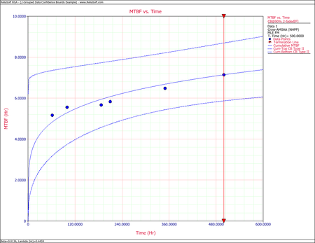
A new helicopter system is under development. System failure data has been collected on five helicopters during the final test phase. The actual failure times cannot be determined since the failures are not discovered until after the helicopters are brought into the maintenance area. However, total flying hours are known when the helicopters are brought in for service, and every 2 weeks each helicopter undergoes a thorough inspection to uncover any failures that may have occurred since the last inspection. Therefore, the cumulative total number of flight hours and the cumulative total number of failures for the 5 helicopters are known for each 2-week period. The total number of flight hours from the test phase is 500, which was accrued over a period of 12 weeks (six 2-week intervals). For each 2-week interval, the total number of flight hours and total number of failures for the 5 helicopters were recorded. The grouped data set is displayed in the following table.

Grouped Data for a New Helicopter System

Interval	Interval Length	Failures in Interval
1	0 - 62	12
2	62 -100	6
3	100 - 187	15
4	187 - 210	3
5	210 - 350	18
6	350 - 500	16

Do the following:

1. Estimate the parameters of the Crow-AMSAA model using maximum likelihood estimation.
2. Calculate the confidence bounds on the cumulative and instantaneous MTBF using the Fisher Matrix and Crow methods.

Solution

1. Using RGA, the value of [math]\displaystyle{ \hat{\beta }\,\! }[/math], must be solved numerically. Once [math]\displaystyle{ \hat{\beta }\,\! }[/math] has been estimated then the value of [math]\displaystyle{ \hat{\lambda }\,\! }[/math] can be determined. The parameter values are displayed below:

   [math]\displaystyle{ \hat{\beta }= 0.81361\,\! }[/math]

   [math]\displaystyle{ \hat{\lambda }= 0.44585\,\! }[/math]

   The grouped Fisher Matrix confidence bounds can be obtained on the parameters [math]\displaystyle{ \hat{\beta }\,\! }[/math] and [math]\displaystyle{ \hat{\lambda }\,\! }[/math] at the 90% confidence level by:

   [math]\displaystyle{ \begin{align} {{\beta }_{L}} = & \hat{\beta }{{e}^{{{z}_{\alpha }}\sqrt{Var(\hat{\beta })}/\hat{\beta }}} \\ = & 0.6546 \\ {{\beta }_{U}} = & \hat{\beta }{{e}^{-{{z}_{\alpha }}\sqrt{Var(\hat{\beta })}/\hat{\beta }}} \\ = & 1.0112 \end{align}\,\! }[/math]

   and:

   [math]\displaystyle{ \begin{align} {{\lambda }_{L}} = & \hat{\lambda }{{e}^{{{z}_{\alpha }}\sqrt{Var(\hat{\lambda })}/\hat{\lambda }}} \\ = & 0.14594 \\ {{\lambda }_{U}} = & \hat{\lambda }{{e}^{-{{z}_{\alpha }}\sqrt{Var(\hat{\lambda })}/\hat{\lambda }}} \\ = & 1.36207 \end{align}\,\! }[/math]

   Crow confidence bounds can also be obtained on the parameters [math]\displaystyle{ \hat{\beta }\,\! }[/math] and [math]\displaystyle{ \hat{\lambda }\,\! }[/math] at the 90% confidence level, as:

   [math]\displaystyle{ \begin{align} {{\beta }_{L}} = & \hat{\beta }(1-S) \\ = & 0.63552 \\ {{\beta }_{U}} = & \hat{\beta }(1+S) \\ = & 0.99170 \end{align}\,\! }[/math]

   and:

   [math]\displaystyle{ \begin{align} {{\lambda }_{L}} = & \frac{\chi _{\tfrac{\alpha }{2},2N}^{2}}{2\cdot T_{k}^{\beta }} \\ = & 0.36197 \\ {{\lambda }_{U}} = & \frac{\chi _{1-\tfrac{\alpha }{2},2N+2}^{2}}{2\cdot T_{k}^{\beta }} \\ = & 0.53697 \end{align}\,\! }[/math]

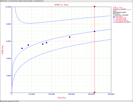
2. The Fisher Matrix confidence bounds for the cumulative MTBF and the instantaneous MTBF at the 90% 2-sided confidence level and for [math]\displaystyle{ T=500\,\! }[/math] hour are:

   [math]\displaystyle{ \begin{align} {{[{{m}_{c}}(T)]}_{L}} = & {{{\hat{m}}}_{c}}(t){{e}^{{{z}_{\alpha /2}}\sqrt{Var({{{\hat{m}}}_{c}}(t))}/{{{\hat{m}}}_{c}}(t)}} \\ = & 5.8680 \\ {{[{{m}_{c}}(T)]}_{U}} = & {{{\hat{m}}}_{c}}(t){{e}^{-{{z}_{\alpha /2}}\sqrt{Var({{{\hat{m}}}_{c}}(t))}/{{{\hat{m}}}_{c}}(t)}} \\ = & 8.6947 \end{align}\,\! }[/math]

   and:

   [math]\displaystyle{ \begin{align} {{[MTB{{F}_{i}}]}_{L}} = & {{{\hat{m}}}_{i}}(t){{e}^{{{z}_{\alpha /2}}\sqrt{Var({{{\hat{m}}}_{i}}(t))}/{{{\hat{m}}}_{i}}(t)}} \\ = & 6.6483 \\ {{[MTB{{F}_{i}}]}_{U}} = & {{{\hat{m}}}_{i}}(t){{e}^{-{{z}_{\alpha /2}}\sqrt{Var({{{\hat{m}}}_{i}}(t))}/{{{\hat{m}}}_{i}}(t)}} \\ = & 11.5932 \end{align}\,\! }[/math]

   The next two figures show plots of the Fisher Matrix confidence bounds for the cumulative and instantaneous MTBF.
   
   

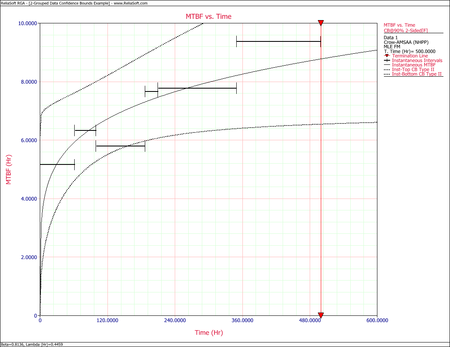
   The Crow confidence bounds for the cumulative and instantaneous MTBF at the 90% 2-sided confidence level and for [math]\displaystyle{ T = 500\,\! }[/math]hours are:

   [math]\displaystyle{ \begin{align} {{[{{m}_{c}}(T)]}_{L}} = & \frac{1}{C{{(t)}_{U}}} \\ = & 5.85449 \\ {{[{{m}_{c}}(T)]}_{U}} = & \frac{1}{C{{(t)}_{L}}} \\ = & 8.79822 \end{align}\,\! }[/math]

   and:

   [math]\displaystyle{ \begin{align} {{[MTB{{F}_{i}}]}_{L}} = & {{\hat{m}}_{i}}(1-W) \\ = & 6.19623 \\ {{[MTB{{F}_{i}}]}_{U}} = & {{\hat{m}}_{i}}(1+W) \\ = & 11.36223 \end{align}\,\! }[/math]

   The next two figures show plots of the Crow confidence bounds for the cumulative and instantaneous MTBF.

   
   

Goodness-of-Fit Tests

Goodness-of-Fit Tests

Missing Data

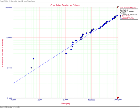
Most of the reliability growth models used for estimating and tracking reliability growth based on test data assume that the data set represents all actual system failure times consistent with a uniform definition of failure (complete data). In practice, this may not always be the case and may result in too few or too many failures being reported over some interval of test time. This may result in distorted estimates of the growth rate and current system reliability. This section discusses a practical reliability growth estimation and analysis procedure based on the assumption that anomalies may exist within the data over some interval of the test period but the remaining failure data follows the Crow-AMSAA reliability growth model. In particular, it is assumed that the beginning and ending points in which the anomalies lie are generated independently of the underlying reliability growth process. The approach for estimating the parameters of the growth model with problem data over some interval of time is basically to not use this failure information. The analysis retains the contribution of the interval to the total test time, but no assumptions are made regarding the actual number of failures over the interval. This is often referred to as gap analysis.

Consider the case where a system is tested for time [math]\displaystyle{ T\,\! }[/math] and the actual failure times are recorded. The time [math]\displaystyle{ T\,\! }[/math] may possibly be an observed failure time. Also, the end points of the gap interval may or may not correspond to a recorded failure time. The underlying assumption is that the data used in the maximum likelihood estimation follows the Crow-AMSAA model with a Weibull intensity function [math]\displaystyle{ \lambda \beta {{t}^{\beta -1}}\,\! }[/math]. It is not assumed that zero failures occurred during the gap interval, rather, it is assumed that the actual number of failures is unknown, and hence no information at all regarding these failure is used to estimate [math]\displaystyle{ \lambda \,\! }[/math] and [math]\displaystyle{ \beta \,\! }[/math].

Let [math]\displaystyle{ {{S}_{1}}\,\! }[/math], [math]\displaystyle{ {{S}_{2}}\,\! }[/math] denote the end points of the gap interval, [math]\displaystyle{ {{S}_{1}}\lt {{S}_{2}}.\,\! }[/math] Let [math]\displaystyle{ 0\lt {{X}_{1}}\lt {{X}_{2}}\lt \ldots \lt {{X}_{{{N}_{1}}}}\le {{S}_{1}}\,\! }[/math] be the failure times over [math]\displaystyle{ (0,\,{{S}_{1}})\,\! }[/math] and let [math]\displaystyle{ {{S}_{2}}\lt {{Y}_{1}}\lt {{Y}_{2}}\lt \ldots \lt {{Y}_{{{N}_{1}}}}\le T\,\! }[/math] be the failure times over [math]\displaystyle{ ({{S}_{2}},\,T)\,\! }[/math]. The maximum likelihood estimates of [math]\displaystyle{ \lambda \,\! }[/math] and [math]\displaystyle{ \beta \,\! }[/math] are values [math]\displaystyle{ \widehat{\lambda }\,\! }[/math] and [math]\displaystyle{ \widehat{\beta }\,\! }[/math] satisfying the following equations.

[math]\displaystyle{ \widehat{\lambda }=\frac{{{N}_{1}}+{{N}_{2}}}{S\widehat{_{1}^{\beta }}+{{T}^{\widehat{\beta }}}-S_{2}^{\widehat{\beta }}}\,\! }[/math]

[math]\displaystyle{ \widehat{\beta }=\frac{{{N}_{1}}+{{N}_{2}}}{\widehat{\lambda }\left[ S\widehat{_{1}^{\beta }}\ln {{S}_{1}}+{{T}^{\widehat{\beta }}}\ln T-S_{2}^{\widehat{\beta }}\ln {{S}_{2}} \right]-\left[ \underset{i=1}{\overset{{{N}_{1}}}{\mathop{\sum }}}\,\ln {{X}_{i}}+\underset{i=1}{\overset{{{N}_{2}}}{\mathop{\sum }}}\,\ln {{Y}_{i}} \right]}\,\! }[/math]

In general, these equations cannot be solved explicitly for [math]\displaystyle{ \widehat{\lambda }\,\! }[/math] and [math]\displaystyle{ \widehat{\beta }\,\! }[/math], but must be solved by an iterative procedure.

Example - Gap Analysis

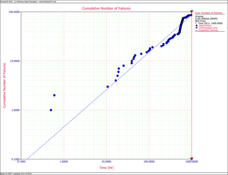
Consider a system under development that was subjected to a reliability growth test for [math]\displaystyle{ T=1,000\,\! }[/math] hours. Each month, the successive failure times, on a cumulative test time basis, were reported. According to the test plan, 125 hours of test time were accumulated on each prototype system each month. The total reliability growth test program lasted for 7 months. One prototype was tested for each of the months 1, 3, 4, 5, 6 and 7 with 125 hours of test time. During the second month, two prototypes were tested for a total of 250 hours of test time. The next table shows the successive [math]\displaystyle{ N=86\,\! }[/math] failure times that were reported for [math]\displaystyle{ T=1,000\,\! }[/math] hours of testing.

[math]\displaystyle{ {{X}_{i}},\,\! }[/math] [math]\displaystyle{ i=1,2,\ldots ,86\,\! }[/math], [math]\displaystyle{ N = 86, T = 1000\,\! }[/math]

.5	.6	10.7	16.6	18.3	19.2	19.5	25.3
39.2	39.4	43.2	44.8	47.4	65.7	88.1	97.2
104.9	105.1	120.8	195.7	217.1	219	257.5	260.4
281.3	283.7	289.8	306.6	328.6	357.0	371.7	374.7
393.2	403.2	466.5	500.9	501.5	518.4	520.7	522.7
524.6	526.9	527.8	533.6	536.5	542.6	543.2	545.0
547.4	554.0	554.1	554.2	554.8	556.5	570.6	571.4
574.9	576.8	578.8	583.4	584.9	590.6	596.1	599.1
600.1	602.5	613.9	616.0	616.2	617.1	621.4	622.6
624.7	628.8	642.4	684.8	731.9	735.1	753.6	792.5
803.7	805.4	832.5	836.2	873.2	975.1

The observed and cumulative number of failures for each month are:

Month	Time Period	Observed Failure Times	Cumulative Failure Times
1	0-125	19	19
2	125-375	13	32
3	375-500	3	35
4	500-625	38	73
5	625-750	5	78
6	750-875	7	85
7	875-1000	1	86

1. Determine the maximum likelihood estimators for the Crow-AMSAA model.
2. Evaluate the goodness-of-fit for the model.
3. Consider [math]\displaystyle{ (500,\ 625)\,\! }[/math] as the gap interval and determine the maximum likelihood estimates of [math]\displaystyle{ \lambda \,\! }[/math] and [math]\displaystyle{ \beta \,\! }[/math].

Solution

1. For the time terminated test:

   [math]\displaystyle{ \begin{align} & \widehat{\beta }= & 0.7597 \\ & \widehat{\lambda }= & 0.4521 \end{align}\,\! }[/math]

2. The Cramér-von Mises goodness-of-fit test for this data set yields:

   [math]\displaystyle{ C_{M}^{2}=\tfrac{1}{12M}+\underset{i=1}{\overset{M}{\mathop{\sum }}}\,{{\left[ (\tfrac{{{T}_{i}}}{T})\widehat{^{\beta }}-\tfrac{2i-1}{2M} \right]}^{2}}= 0.6989\,\! }[/math]

   The critical value at the 10% significance level is 0.173. Therefore, the test indicated that the analyst should reject the hypothesis that the data set follows the Crow-AMSAA reliability growth model. The following plot shows [math]\displaystyle{ \ln N(t)\,\! }[/math] versus [math]\displaystyle{ \ln t\,\! }[/math] with the fitted line [math]\displaystyle{ \ln \hat{\lambda }+\hat{\beta }\ln t\,\! }[/math], where [math]\displaystyle{ \widehat{\lambda }=0.4521\,\! }[/math] and [math]\displaystyle{ \widehat{\beta }=0.7597\,\! }[/math] are the maximum likelihood estimates.
   

   Observing the data during the fourth month (between 500 and 625 hours), 38 failures were reported. This number is very high in comparison to the failures reported in the other months. A quick investigation found that a number of new data collectors were assigned to the project during this month. It was also discovered that extensive design changes were made during this period, which involved the removal of a large number of parts. It is possible that these removals, which were not failures, were incorrectly reported as failed parts. Based on knowledge of the system and the test program, it was clear that such a large number of actual system failures was extremely unlikely. The consensus was that this anomaly was due to the failure reporting. For this analysis, it was decided that the actual number of failures over this month is assumed to be unknown, but consistent with the remaining data and the Crow-AMSAA reliability growth model.

3. Considering the problem interval [math]\displaystyle{ (500,625)\,\! }[/math] as the gap interval, we will use the data over the interval [math]\displaystyle{ (0,500)\,\! }[/math] and over the interval [math]\displaystyle{ (625,1000).\,\! }[/math] The equations for analyzing missing data are the appropriate equations to estimate [math]\displaystyle{ \lambda \,\! }[/math] and [math]\displaystyle{ \beta \,\! }[/math] because the failure times are known. In this case [math]\displaystyle{ {{S}_{1}}=500,\,{{S}_{2}}=625\,\! }[/math] and [math]\displaystyle{ T=1000,\ {{N}_{1}}=35,\,{{N}_{2}}=13\,\! }[/math]. The maximum likelihood estimates of [math]\displaystyle{ \lambda \,\! }[/math] and [math]\displaystyle{ \beta \,\! }[/math] are:

   [math]\displaystyle{ \begin{align} & \widehat{\beta }= & 0.5596 \\ & \widehat{\lambda }= & 1.1052 \end{align}\,\! }[/math]

   The next figure is a plot of the cumulative number of failures versus time. This plot is approximately linear, which also indicates a good fit of the model.
   

Crow Discrete Reliability Growth Model

The Crow-AMSAA model can be adapted for the analysis of success/failure data (also called discrete or attribute data). Suppose system development is represented by [math]\displaystyle{ i\,\! }[/math] configurations. This corresponds to [math]\displaystyle{ i-1\,\! }[/math] configuration changes, unless fixes are applied at the end of the test phase, in which case there would be [math]\displaystyle{ i\,\! }[/math] configuration changes. Let [math]\displaystyle{ {{N}_{i}}\,\! }[/math] be the number of trials during configuration [math]\displaystyle{ i\,\! }[/math] and let [math]\displaystyle{ {{M}_{i}}\,\! }[/math] be the number of failures during configuration [math]\displaystyle{ i\,\! }[/math]. Then the cumulative number of trials through configuration [math]\displaystyle{ i\,\! }[/math], namely [math]\displaystyle{ {{T}_{i}}\,\! }[/math], is the sum of the [math]\displaystyle{ {{N}_{i}}\,\! }[/math] for all [math]\displaystyle{ i\,\! }[/math], or:

[math]\displaystyle{ {{T}_{i}}=\underset{}{\overset{}{\mathop \sum }}\,{{N}_{i}}\,\! }[/math]

And the cumulative number of failures through configuration [math]\displaystyle{ i\,\! }[/math], namely [math]\displaystyle{ {{K}_{i}}\,\! }[/math], is the sum of the [math]\displaystyle{ {{M}_{i}}\,\! }[/math] for all [math]\displaystyle{ i\,\! }[/math], or:

[math]\displaystyle{ {{K}_{i}}=\underset{}{\overset{}{\mathop \sum }}\,{{M}_{i}}\,\! }[/math]

The expected value of [math]\displaystyle{ {{K}_{i}}\,\! }[/math] can be expressed as [math]\displaystyle{ E[{{K}_{i}}]\,\! }[/math] and defined as the expected number of failures by the end of configuration [math]\displaystyle{ i\,\! }[/math]. Applying the learning curve property to [math]\displaystyle{ E[{{K}_{i}}]\,\! }[/math] implies:

[math]\displaystyle{ E\left[ {{K}_{i}} \right]=\lambda T_{i}^{\beta }\,\! }[/math]

Denote [math]\displaystyle{ {{f}_{1}}\,\! }[/math] as the probability of failure for configuration 1 and use it to develop a generalized equation for [math]\displaystyle{ {{f}_{i}}\,\! }[/math] in terms of the [math]\displaystyle{ {{T}_{i}}\,\! }[/math] and [math]\displaystyle{ {{N}_{i}}\,\! }[/math]. From the equation above, the expected number of failures by the end of configuration 1 is:

[math]\displaystyle{ E\left[ {{K}_{1}} \right]=\lambda T_{1}^{\beta }={{f}_{1}}{{N}_{1}}\,\! }[/math]

[math]\displaystyle{ \therefore {{f}_{1}}=\frac{\lambda T_{1}^{\beta }}{{{N}_{1}}}\,\! }[/math]

Applying the [math]\displaystyle{ E\left[ {{K}_{i}}\right]\,\! }[/math] equation again and noting that the expected number of failures by the end of configuration 2 is the sum of the expected number of failures in configuration 1 and the expected number of failures in configuration 2:

[math]\displaystyle{ \begin{align} E\left[ {{K}_{2}} \right] = & \lambda T_{2}^{\beta } \\ = & {{f}_{1}}{{N}_{1}}+{{f}_{2}}{{N}_{2}} \\ = & \lambda T_{1}^{\beta }+{{f}_{2}}{{N}_{2}} \end{align}\,\! }[/math]

[math]\displaystyle{ \therefore {{f}_{2}}=\frac{\lambda T_{2}^{\beta }-\lambda T_{1}^{\beta }}{{{N}_{2}}}\,\! }[/math]

By this method of inductive reasoning, a generalized equation for the failure probability on a configuration basis, [math]\displaystyle{ {{f}_{i}}\,\! }[/math], is obtained, such that:

[math]\displaystyle{ {{f}_{i}}=\frac{\lambda T_{i}^{\beta }-\lambda T_{i-1}^{\beta }}{{{N}_{i}}}\,\! }[/math]

For the special case where [math]\displaystyle{ {{N}_{i}}=1\,\! }[/math] for all [math]\displaystyle{ i\,\! }[/math], the equation above becomes a smooth curve, [math]\displaystyle{ {{g}_{i}}\,\! }[/math], that represents the probability of failure for trial by trial data, or:

[math]\displaystyle{ {{g}_{i}}=\lambda \cdot {{i}^{\beta }}-\lambda \cdot {{\left( i-1 \right)}^{\beta }}\,\! }[/math]

In this equation, [math]\displaystyle{ i\,\! }[/math] represents the trial number. Thus an equation for the reliability (probability of success) for the [math]\displaystyle{ {{i}^{th}}\,\! }[/math] configuration is obtained:

[math]\displaystyle{ \begin{align} {{R}_{i}}=1-{{f}_{i}} \end{align}\,\! }[/math]

The equation for the reliability for the [math]\displaystyle{ {{i}^{th}}\,\! }[/math] trial is:

[math]\displaystyle{ \begin{align} {{R}_{i}}=1-{{g}_{i}} \end{align}\,\! }[/math]

Maximum Likelihood Estimators for Discrete Model

This section describes procedures for estimating the parameters of the Crow-AMSAA model for success/failure data. An example is presented illustrating these concepts. The estimation procedures provide maximum likelihood estimates (MLEs) for the model's two parameters, [math]\displaystyle{ \lambda \,\! }[/math] and [math]\displaystyle{ \beta \,\! }[/math]. The MLEs for [math]\displaystyle{ \lambda \,\! }[/math] and [math]\displaystyle{ \beta \,\! }[/math] allow for point estimates for the probability of failure, given by:

[math]\displaystyle{ {{\hat{f}}_{i}}=\frac{\hat{\lambda }T_{i}^{{\hat{\beta }}}-\hat{\lambda }T_{i-1}^{{\hat{\beta }}}}{{{N}_{i}}}=\frac{\hat{\lambda }\left( T_{i}^{{\hat{\beta }}}-T_{i-1}^{{\hat{\beta }}} \right)}{{{N}_{i}}}\,\! }[/math]

And the probability of success (reliability) for each configuration [math]\displaystyle{ i\,\! }[/math] is equal to:

[math]\displaystyle{ {{\hat{R}}_{i}}=1-{{\hat{f}}_{i}}\,\! }[/math]

The likelihood function is:

[math]\displaystyle{ \underset{i=1}{\overset{k}{\mathop \prod }}\,\left( \begin{matrix} {{N}_{i}} \\ {{M}_{i}} \\ \end{matrix} \right){{\left( \frac{\lambda T_{i}^{\beta }-\lambda T_{i-1}^{\beta }}{{{N}_{i}}} \right)}^{{{M}_{i}}}}{{\left( \frac{{{N}_{i}}-\lambda T_{i}^{\beta }+\lambda T_{i-1}^{\beta }}{{{N}_{i}}} \right)}^{{{N}_{i}}-{{M}_{i}}}}\,\! }[/math]

Taking the natural log on both sides yields:

[math]\displaystyle{ \begin{align} & \Lambda = & \underset{i=1}{\overset{K}{\mathop \sum }}\,\left[ \ln \left( \begin{matrix} {{N}_{i}} \\ {{M}_{i}} \\ \end{matrix} \right)+{{M}_{i}}\left[ \ln (\lambda T_{i}^{\beta }-\lambda T_{i-1}^{\beta })-\ln {{N}_{i}} \right] \right] \\ & & +\underset{i=1}{\overset{K}{\mathop \sum }}\,\left[ ({{N}_{i}}-{{M}_{i}})\left[ \ln ({{N}_{i}}-\lambda T_{i}^{\beta }+\lambda T_{i-1}^{\beta })-\ln {{N}_{i}} \right] \right] \end{align}\,\! }[/math]

Taking the derivative with respect to [math]\displaystyle{ \lambda \,\! }[/math] and [math]\displaystyle{ \beta \,\! }[/math] respectively, exact MLEs for [math]\displaystyle{ \lambda \,\! }[/math] and [math]\displaystyle{ \beta \,\! }[/math] are values satisfying the following two equations:

[math]\displaystyle{ \begin{align} & \underset{i=1}{\overset{K}{\mathop \sum }}\,{{H}_{i}}\times {{S}_{i}}= & 0 \\ & \underset{i=1}{\overset{K}{\mathop \sum }}\,{{U}_{i}}\times {{S}_{i}}= & 0 \end{align}\,\! }[/math]

where:

[math]\displaystyle{ \begin{align} {{H}_{i}}= & \underset{i=1}{\overset{K}{\mathop \sum }}\,\left[ T_{i}^{\beta }\ln {{T}_{i}}-T_{i-1}^{\beta }\ln {{T}_{i-1}} \right] \\ {{S}_{i}}= & \frac{{{M}_{i}}}{\left[ \lambda T_{i}^{\beta }-\lambda T_{i-1}^{\beta } \right]}-\frac{{{N}_{i}}-{{M}_{i}}}{\left[ {{N}_{i}}-\lambda T_{i}^{\beta }+\lambda T_{i-1}^{\beta } \right]} \\ {{U}_{i}}= & T_{i}^{\beta }-T_{i-1}^{\beta }\, \end{align}\,\! }[/math]

Discrete Model Example

A one-shot system underwent reliability growth development testing for a total of 68 trials. Delayed corrective actions were incorporated after the 14th, 33rd and 48th trials. From trial 49 to trial 68, the configuration was not changed.

• Configuration 1 experienced 5 failures,
• Configuration 2 experienced 3 failures,
• Configuration 3 experienced 4 failures and
• Configuration 4 experienced 4 failures.

Do the following:

1. Estimate the parameters of the Crow-AMSAA model using maximum likelihood estimation.
2. Estimate the unreliability and reliability by configuration.

Solution

1. The parameter estimates for the Crow-AMSAA model using the parameter estimation for discrete data methodology yields [math]\displaystyle{ \lambda = 0.5954\,\! }[/math] and [math]\displaystyle{ \beta =0.7801\,\! }[/math].
2. The following table displays the results for probability of failure and reliability, and these results are displayed in the next two plots. Estimated Failure Probability and Reliability by Configuration

   Configuration([math]\displaystyle{ i\,\! }[/math])	Estimated Failure Probability	Estimated Reliability
   1	0.333	0.667
   2	0.234	0.766
   3	0.206	0.794
   4	0.190	0.810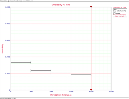

   
   

Discrete Model for Mixed Data

In the RGA software, the Discrete Data > Mixed Data option gives a data sheet that can have input data that is either a configuration in groups or individual trial by trial, or a mixed combination of individual trials and configurations of more than one trial. The calculations use the same mathematical methods described in the Grouped Data section.

Mixed Data Example

The table below shows the number of failures of each interval of trials and the cumulative number of trials in each interval for a reliability growth test. For example, the first row indicates that for an interval of 14 trials, 5 failures occurred.

Mixed Data

Failures in Interval	Cumulative Trials
5	14
3	33
4	48
0	52
1	53
0	57
1	58
0	62
1	63
0	67
1	68

Using the RGA software, the parameters of the Crow-AMSAA model are estimated as follows:

[math]\displaystyle{ \hat{\beta }=0.7950\,\! }[/math]

and:

[math]\displaystyle{ \hat{\lambda }=0.5588\,\! }[/math]

As we have seen, the Crow-AMSAA instantaneous failure intensity, [math]\displaystyle{ {{\lambda }_{i}}(T)\,\! }[/math], is defined as:

[math]\displaystyle{ \begin{align} {{\lambda }_{i}}(T)=\lambda \beta {{T}^{\beta -1}},\text{with }T\gt 0,\text{ }\lambda \gt 0\text{ and }\beta \gt 0 \end{align}\,\! }[/math]

Using the parameter estimates, we can calculate the instantaneous unreliability at the end of the test, or [math]\displaystyle{ T=68.\,\! }[/math]

[math]\displaystyle{ {{R}_{i}}(68)=0.5588\cdot 0.7950\cdot {{68}^{0.7950-1}}=0.1871\,\! }[/math]

This result that can be obtained from the Quick Calculation Pad (QCP), for [math]\displaystyle{ T=68,\,\! }[/math] as seen in the following picture.

The instantaneous reliability can then be calculated as:

[math]\displaystyle{ \begin{align} {{R}_{inst}}=1-0.1871=0.8129 \end{align}\,\! }[/math]

Mixed Data Confidence Bounds

Bounds on Average Failure Probability for Mixed Data
The process to calculate the average unreliability confidence bounds for mixed data is as follows:

1) Calculate the average failure probability [math]\displaystyle{ ({{t}_{1}},{{t}_{2}})\,\! }[/math].

2) There will exist a [math]\displaystyle{ {{t}^{*}}\,\! }[/math] between [math]\displaystyle{ {{t}_{1}}\,\! }[/math] and [math]\displaystyle{ {{t}_{2}}\,\! }[/math] such that the instantaneous unreliability at [math]\displaystyle{ {{t}^{*}}\,\! }[/math] equals the average unreliability [math]\displaystyle{ ({{t}_{1}},{{t}_{2}})\,\! }[/math]. The confidence intervals for the instantaneous unreliability at [math]\displaystyle{ {{t}^{*}}\,\! }[/math] are the confidence intervals for the average unreliability [math]\displaystyle{ ({{t}_{1}},{{t}_{2}})\,\! }[/math].

Bounds on Average Reliability for Mixed Data
The process to calculate the average reliability confidence bounds for mixed data is as follows:

1) Calculate confidence bounds for average unreliability [math]\displaystyle{ ({{t}_{1}},{{t}_{2}})\,\! }[/math] as described above.

2) The confidence bounds for reliability are 1 minus these confidence bounds for average unreliability.

Change of Slope

The assumption of the Crow-AMSAA (NHPP) model is that the failure intensity is monotonically increasing, decreasing or remaining constant over time. However, there might be cases in which the system design or the operational environment experiences major changes during the observation period and, therefore, a single model will not be appropriate to describe the failure behavior for the entire timeline. RGA incorporates a methodology that can be applied to scenarios where a major change occurs during a reliability growth test. The test data can be broken into two segments with a separate Crow-AMSAA (NHPP) model applied to each segment.

Consider the data in the following plot from a reliability growth test.

As discussed above, the cumulative number of failures vs. the cumulative time should be linear on logarithmic scales. The next figure shows the data plotted on logarithmic scales.

One can easily recognize that the failure behavior is not constant throughout the duration of the test. Just by observing the data, it can be asserted that a major change occurred at around 140 hours that resulted in a change in the rate of failures. Therefore, using a single model to analyze this data set likely will not be appropriate.

The Change of Slope methodology proposes to split the data into two segments and apply a Crow-AMSAA (NHPP) model to each segment. The time of change that will be used to split the data into the two segments (it will be referred to as [math]\displaystyle{ {{T}_{1}}\,\! }[/math] ) could be estimated just by observing the data, but will most likely be dictated by engineering knowledge of the specific change to the system design or operating conditions. It is important to note that although two separate models will be applied to each segment, the information collected in the first segment (i.e., data up to [math]\displaystyle{ {{T}_{1}}\,\! }[/math] ) will be considered when creating the model for the second segment (i.e., data after [math]\displaystyle{ {{T}_{1}}\,\! }[/math] ). The models presented next can be applied to the reliability growth analysis of a single system or multiple systems.

Model for First Segment (Data up to T₁)

The data up to the point of the change that occurs at [math]\displaystyle{ {{T}_{1}}\,\! }[/math] will be analyzed using the Crow-AMSAA (NHPP) model. Based on the ML equations for [math]\displaystyle{ \lambda \,\! }[/math] and [math]\displaystyle{ \beta \,\! }[/math] (in the section Maximum Likelihood Estimators), the ML estimators of the model are:

[math]\displaystyle{ \widehat{{{\lambda }_{1}}}=\frac{{{n}_{1}}}{T_{1}^{{{\beta }_{1}}}}\,\! }[/math]

and

[math]\displaystyle{ {{\widehat{\beta }}_{1}}=\frac{{{n}_{1}}}{{{n}_{1}}\ln {{T}_{1}}-\underset{i=1}{\overset{{{n}_{1}}}{\mathop{\sum }}}\,\ln {{t}_{i}}}\,\! }[/math]

where:

• [math]\displaystyle{ {{T}_{1}}\,\! }[/math] is the time when the change occurs
• [math]\displaystyle{ {{n}_{1}}\,\! }[/math] is the number of failures observed up to time [math]\displaystyle{ {{T}_{1}}\,\! }[/math]
• [math]\displaystyle{ {{t}_{i}}\,\! }[/math] is the time at which each corresponding failure was observed

The equation for [math]\displaystyle{ \widehat{\beta_{1}}\,\! }[/math] can be rewritten as follows:

[math]\displaystyle{ \begin{align} {{\widehat{\beta }}_{1}}= & \frac{{{n}_{1}}}{{{n}_{1}}\ln {{T}_{1}}-\left( \ln {{t}_{1}}+\ln {{t}_{2}}+...+\ln {{t}_{{{n}_{1}}}} \right)} \\ = & \frac{{{n}_{1}}}{(\ln {{T}_{1}}-\ln {{t}_{1}})+(\ln {{T}_{1}}-\ln {{t}_{2}})+(...)+(\ln {{T}_{1}}-\ln {{t}_{{{n}_{1}}}})} \\ = & \frac{{{n}_{1}}}{\ln \tfrac{{{T}_{1}}}{{{t}_{1}}}+\ln \tfrac{{{T}_{1}}}{{{t}_{2}}}+...+\ln \tfrac{{{T}_{1}}}{{{t}_{{{n}_{1}}}}}} \end{align}\,\! }[/math]

or

[math]\displaystyle{ {{\widehat{\beta }}_{1}}=\frac{{{n}_{1}}}{\underset{i=1}{\overset{{{n}_{1}}}{\mathop{\sum }}}\,\ln \tfrac{{{T}_{1}}}{{{t}_{i}}}}\,\! }[/math]

Model for Second Segment (Data after T₁)

The Crow-AMSAA (NHPP) model will be used again to analyze the data after [math]\displaystyle{ {{T}_{1}}\,\! }[/math]. However, the information collected during the first segment will be used when creating the model for the second segment. Given that, the ML estimators of the model parameters in the second segment are:

[math]\displaystyle{ \widehat{{{\lambda }_{2}}}=\frac{{{n}}}{T_{2}^{{{\beta }_{2}}}}\,\! }[/math]

and:

[math]\displaystyle{ {{\widehat{\beta }}_{2}}=\frac{{{n}_{2}}}{{{n}_{1}}\ln \tfrac{{{T}_{2}}}{{{T}_{1}}}+\underset{i={{n}_{1}}+1}{\overset{n}{\mathop{\sum }}}\,\ln \tfrac{{{T}_{2}}}{{{t}_{i}}}}\,\! }[/math]

where:

• [math]\displaystyle{ {{n}_{2}}\,\! }[/math] is the number of failures that were observed after [math]\displaystyle{ {{T}_{1}}\,\! }[/math]
• [math]\displaystyle{ n={{n}_{1}}+{{n}_{2}}\,\! }[/math] is the total number of failures observed throughout the test
• [math]\displaystyle{ {{T}_{2}}\,\! }[/math] is the end time of the test. The test can either be failure terminated or time terminated

Example - Multiple MLE

The following table gives the failure times obtained from a reliability growth test of a newly designed system. The test has a duration of 660 hours.

Failure Times From a Reliability Growth Test [math]\displaystyle{ \begin{matrix} \text{7}\text{.8} & \text{99}\text{.2} & \text{151} & \text{260}\text{.1} & \text{342} & \text{430}\text{.2} \\ \text{17}\text{.6} & \text{99}\text{.6} & \text{163} & \text{273}\text{.1} & \text{350}\text{.2} & \text{445}\text{.7} \\ \text{25}\text{.3} & \text{100}\text{.3} & \text{174}\text{.5} & \text{274}\text{.7} & \text{355}\text{.2} & \text{475}\text{.9} \\ \text{15} & \text{102}\text{.5} & \text{177}\text{.4} & \text{282}\text{.8} & \text{364}\text{.6} & \text{490}\text{.1} \\ \text{47}\text{.5} & \text{112} & \text{191}\text{.6} & \text{285} & \text{364}\text{.9} & \text{535} \\ \text{54} & \text{112}\text{.2} & \text{192}\text{.7} & \text{315}\text{.4} & \text{366}\text{.3} & \text{580}\text{.3} \\ \text{54}\text{.5} & \text{120}\text{.9} & \text{213} & \text{317}\text{.1} & \text{379}\text{.4} & \text{610}\text{.6} \\ \text{56}\text{.4} & \text{121}\text{.9} & \text{244}\text{.8} & \text{320}\text{.6} & \text{389} & \text{640}\text{.5} \\ \text{63}\text{.6} & \text{125}\text{.5} & \text{249} & \text{324}\text{.5} & \text{394}\text{.9} & {} \\ \text{72}\text{.2} & \text{133}\text{.4} & \text{250}\text{.8} & \text{324}\text{.9} & \text{395}\text{.2} & {} \\ \end{matrix}\,\! }[/math]

First, apply a single Crow-AMSAA (NHPP) model to all of the data. The following plot shows the expected failures obtained from the model (the line) along with the observed failures (the points).

The plot shows that the model does not seem to accurately track the data. This is confirmed by performing the Cramér-von Mises goodness-of-fit test, which checks the hypothesis that the data follows a non-homogeneous Poisson process with a power law failure intensity. The model fails the goodness-of-fit test because the test statistic (0.3309) is higher than the critical value (0.1729) at the 0.1 significance level. The next figure shows a customized report that displays both the calculated parameters and the statistical test results.

Through further investigation, it is discovered that a significant design change occurred at 400 hours of test time. It is suspected that this modification is responsible for the change in the failure behavior.

In RGA, you have the option to perform a standard Crow-AMSAA (NHPP) analysis, or perform a Change of Slope analysis where you specify a specific breakpoint, as shown in the following figure. RGA actually creates a grouped data set where the data in Segment 1 is included and defined by a single interval to calculate the Segment 2 parameters. However, these results are equivalent to the parameters estimated using the equations presented here.

Therefore, the Change of Slope methodology is applied to break the data into two segments for analysis. The first segment is set from 0 to 400 hours and the second segment is from 401 to 660 hours (which is the end time of the test). The Crow-AMSAA (NHPP) parameters for the first segment (0-400 hours) are:

[math]\displaystyle{ \widehat{{{\lambda }_{1}}}=\frac{{{n}_{1}}}{T_{1}^{{{\beta }_{1}}}}=\frac{50}{{{400}^{1.0359}}}=0.1008\,\! }[/math]

and

[math]\displaystyle{ {{\widehat{\beta }}_{1}}=\frac{{{n}_{1}}}{\underset{i=1}{\overset{{{n}_{1}}}{\mathop{\sum }}}\,\ln \tfrac{{{T}_{1}}}{{{t}_{i}}}}=\frac{50}{\underset{i=1}{\overset{50}{\mathop{\sum }}}\,\ln \tfrac{400}{{{t}_{i}}}}=1.0359\,\! }[/math]

The Crow-AMSAA (NHPP) parameters for the second segment (401-660 hours) are:

[math]\displaystyle{ \widehat{{{\lambda }_{2}}}=\frac{{{n}}}{T_{2}^{{{\beta }_{2}}}}=\frac{58}{{{660}^{0.2971}}}=8.4304\,\! }[/math]

[math]\displaystyle{ {{\widehat{\beta }}_{2}}=\frac{{{n}_{2}}}{{{n}_{1}}\ln \tfrac{{{T}_{2}}}{{{T}_{1}}}+\underset{i={{n}_{1}}+1}{\overset{n}{\mathop{\sum }}}\,\ln \tfrac{{{T}_{2}}}{{{t}_{i}}}}=\frac{8}{50\ln \tfrac{660}{400}+\underset{i=51}{\overset{58}{\mathop{\sum }}}\,\ln \tfrac{660}{{{T}_{i}}}}=0.2971\,\! }[/math]

The following figure shows a plot of the two-segment analysis along with the observed data. It is obvious that the Change of Slope method tracks the data more accurately.

This can also be verified by performing a chi-squared goodness-of-fit test. The chi-squared statistic is 1.2956, which is lower than the critical value of 12.017 at the 0.1 significance level; therefore, the analysis passes the test. The next figure shows a customized report that displays both the calculated parameters and the statistical test results.

When you have a model that fits the data, it can be used to make accurate predictions and calculations. Metrics such as the demonstrated MTBF at the end of the test or the expected number of failures at later times can be calculated. For example, the following plot shows the instantaneous MTBF vs. time, together with the two-sided 90% confidence bounds. Note that confidence bounds are available for the second segment only. For times up to 400 hours, the parameters of the first segment were used to calculate the MTBF, while the parameters of the second segment were used for times after 400 hours. Also note that the number of failures at the end of segment 1 is not assumed to be equal to the number of failures at the start of segment 2. This can result in a visible jump in the plot, as in this example.

The next figure shows the use of the Quick Calculation Pad (QCP) in the RGA software to calculate the Demonstrated MTBF at the end of the test (instantaneous MTBF at time = 660), together with the two-sided 90% confidence bounds. All the calculations were based on the parameters of the second segment.

More Examples

Estimating the Number of Failures if Testing Continues

Six systems were subjected to a reliability growth test and a total of 81 failures were observed. The following table presents the start and end times, along with the times-to-failure for each system. Do the following:

1) Estimate the parameters of the Crow-AMSAA model using maximum likelihood estimation.

2) How many additional failures would be generated if testing continues until 3,000 hours?

Multiple systems (concurrent operating times) Data

System	1	2	3	4	5	6
Start Time	0	0	0	0	0	0
End Time	504	541	454	474	436	500
Times-to-Failure	21	83	26	36	23	7
	29	83	26	306	46	13
	43	83	57	306	127	13
	43	169	64	334	166	31
	43	213	169	354	169	31
	66	299	213	395	213	82
	115	375	231	403	213	109
	159	431	231	448	255	137
	199		231	456	369	166
	202		231	461	374	200
	222		304		380	210
	248		383		415	220
	248					422
	255					437
	286					469
	286					469
	304
	320
	348
	364
	404
	410
	429

Solution

1) The next figure shows the parameters estimated using RGA.

Estimated parameters of the Crow-AMSAA model.

2) The number of failures can be estimated using the Quick Calculation Pad, as shown next. The estimated number of failures at 3,000 hours is equal to 83.2451 and 81 failures were observed during testing. Therefore, the number of additional failures generated if testing continues until 3,000 hours is equal to [math]\displaystyle{ 83.2451-81=2.2451\approx 3\,\! }[/math].

Expected number of failures at 3000 hours.

Determining Whether a Design Meets the MTBF Goal

A prototype of a system was tested at the end of one of its design stages. The test was run for a total of 300 hours and 27 failures were observed. The table below shows the collected data set. The prototype has a design specification of an MTBF equal to 10 hours with a 90% confidence level at 300 hours. Do the following:

1) Estimate the parameters of the Crow-AMSAA model using maximum likelihood estimation.

2) Does the prototype meet the specified goal?

Failure Times Data

2.6	56.5	98.1	190.7
16.5	63.1	101.1	193
16.5	70.6	132	198.7
17	73	142.2	251.9
21.4	77.7	147.7	282.5
29.1	93.9	149	286.1
33.3	95.5	167.2

Solution

1) The next figure shows the parameters estimated using RGA.

2) The instantaneous MTBF with one-sided 90% confidence bounds can be calculated using the Quick Calculation Pad (QCP), as shown next. From the QCP, it is estimated that the lower limit on the MTBF at 300 hours with a 90% confidence level is equal to 10.8170 hours. Therefore, the prototype has met the specified goal.

Analyzing Mixed Data for a One-Shot System

A one-shot system underwent reliability growth development for a total of 50 trials. The test was performed as a combination of configuration in groups and individual trial by trial. The table below shows the data set obtained from the test. The first column specifies the number of failures that occurred in each interval, and the second column shows the cumulative number of trials in that interval. Do the following:

1) Estimate the parameters of the Crow-AMSAA model using maximum likelihood estimators.

2) What are the instantaneous reliability and the 2-sided 90% confidence bounds at the end of the test?

3) Plot the cumulative reliability with 2-sided 90% confidence bounds.

4) If the test was continued for another 25 trials what would the expected number of additional failures be?

Mixed Data

Failures in Interval	Cumulative Trials	Failures in Interval	Cumulative Trials
3	4	1	25
0	5	1	28
4	9	0	32
1	12	2	37
0	13	0	39
1	15	1	40
2	19	1	44
1	20	0	46
1	22	1	49
0	24	0	50

Solution

1) The next figure shows the parameters estimated using RGA.

2) The figure below shows the calculation of the instantaneous reliability with the 2-sided 90% confidence bounds. From the QCP, it is estimated that the instantaneous reliability at stage 50 (or at the end of the test) is 72.70% with an upper and lower 2-sided 90% confidence bound of 82.36% and 39.59%, respectively.

3) The following plot shows the cumulative reliability with the 2-sided 90% confidence bounds.

4) The last figure shows the calculation of the expected number of failures after 75 trials. From the QCP, it is estimated that the cumulative number of failures after 75 trials is [math]\displaystyle{ 26.3770\approx 27\,\! }[/math]. Since 20 failures occurred in the first 50 trials, the estimated number of additional failures is 7.