Crow-AMSAA Confidence Bounds Example: Difference between revisions
No edit summary |
mNo edit summary |
||
| Line 4: | Line 4: | ||
Using the values of <math>\hat{\beta }\,\!</math> and <math>\hat{\lambda }\,\!</math> estimated in the <noinclude>[[Crow-AMSAA (NHPP)#Failure_Times_-_Example_1|Failure Times - Example 1]]</noinclude><includeonly>example given above</includeonly>, calculate the 90% 2-sided confidence bounds on the cumulative and instantaneous failure intensity. | Using the values of <math>\hat{\beta }\,\!</math> and <math>\hat{\lambda }\,\!</math> estimated in the <noinclude>[[Crow-AMSAA (NHPP)#Failure_Times_-_Example_1|Failure Times - Example 1]]</noinclude><includeonly>example given above</includeonly>, calculate the 90% 2-sided confidence bounds on the cumulative and instantaneous failure intensity. | ||
'''Solution''' | '''Solution''' | ||
| Line 12: | Line 11: | ||
The partial derivatives for the Fisher Matrix confidence bounds are: | The partial derivatives for the Fisher Matrix confidence bounds are: | ||
:<math>\begin{align} | |||
\frac{{{\partial }^{2}}\Lambda }{\partial {{\lambda }^{2}}} = & -\frac{22}{{{0.4239}^{2}}}=-122.43 \\ | \frac{{{\partial }^{2}}\Lambda }{\partial {{\lambda }^{2}}} = & -\frac{22}{{{0.4239}^{2}}}=-122.43 \\ | ||
\frac{{{\partial }^{2}}\Lambda }{\partial {{\beta }^{2}}} = & -\frac{22}{{{0.6142}^{2}}}-0.4239\cdot {{620}^{0.6142}}{{(\ln 620)}^{2}}=-967.68 \\ | \frac{{{\partial }^{2}}\Lambda }{\partial {{\beta }^{2}}} = & -\frac{22}{{{0.6142}^{2}}}-0.4239\cdot {{620}^{0.6142}}{{(\ln 620)}^{2}}=-967.68 \\ | ||
\frac{{{\partial }^{2}}\Lambda }{\partial \lambda \partial \beta } = & -{{620}^{0.6142}}\ln 620=-333.64 | \frac{{{\partial }^{2}}\Lambda }{\partial \lambda \partial \beta } = & -{{620}^{0.6142}}\ln 620=-333.64 | ||
\end{align}\,\!</math> | \end{align}\,\!</math> | ||
The Fisher Matrix then becomes: | The Fisher Matrix then becomes: | ||
:<math>\begin{align} | |||
\begin{bmatrix}122.43 & 333.64\\ 333.64 & 967.68\end{bmatrix}^{-1} & = \begin{bmatrix}Var(\hat{\lambda}) & Cov(\hat{\beta},\hat{\lambda})\\ | \begin{bmatrix}122.43 & 333.64\\ 333.64 & 967.68\end{bmatrix}^{-1} & = \begin{bmatrix}Var(\hat{\lambda}) & Cov(\hat{\beta},\hat{\lambda})\\ | ||
Cov(\hat{\beta},\hat{\lambda}) & Var(\hat{\beta})\end{bmatrix} \\ | Cov(\hat{\beta},\hat{\lambda}) & Var(\hat{\beta})\end{bmatrix} \\ | ||
& = \begin{bmatrix} 0.13519969 & -0.046614609\\ -0.046614609 & 0.017105343 \end{bmatrix} | & = \begin{bmatrix} 0.13519969 & -0.046614609\\ -0.046614609 & 0.017105343 \end{bmatrix} | ||
\end{align}\,\!</math> | \end{align}\,\!</math> | ||
For <math>T=620\,\!</math> hours, the partial derivatives of the cumulative and instantaneous failure intensities are: | For <math>T=620\,\!</math> hours, the partial derivatives of the cumulative and instantaneous failure intensities are: | ||
:<math>\begin{align} | |||
\frac{\partial {{\lambda }_{c}}(T)}{\partial \beta }= & \hat{\lambda }{{T}^{\hat{\beta }-1}}\ln (T) \\ | \frac{\partial {{\lambda }_{c}}(T)}{\partial \beta }= & \hat{\lambda }{{T}^{\hat{\beta }-1}}\ln (T) \\ | ||
= & 0.4239\cdot {{620}^{-0.3858}}\ln 620 \\ | = & 0.4239\cdot {{620}^{-0.3858}}\ln 620 \\ | ||
| Line 39: | Line 36: | ||
\end{align}\,\!</math> | \end{align}\,\!</math> | ||
:<math>\begin{align} | |||
\frac{\partial {{\lambda }_{i}}(T)}{\partial \beta }= & \hat{\lambda }{{T}^{\hat{\beta }-1}}+\hat{\lambda }\hat{\beta }{{T}^{\hat{\beta }-1}}\ln T \\ | \frac{\partial {{\lambda }_{i}}(T)}{\partial \beta }= & \hat{\lambda }{{T}^{\hat{\beta }-1}}+\hat{\lambda }\hat{\beta }{{T}^{\hat{\beta }-1}}\ln T \\ | ||
= & 0.4239\cdot {{620}^{-0.3858}}+0.4239\cdot 0.6142\cdot {{620}^{-0.3858}}\ln 620 \\ | = & 0.4239\cdot {{620}^{-0.3858}}+0.4239\cdot 0.6142\cdot {{620}^{-0.3858}}\ln 620 \\ | ||
| Line 46: | Line 42: | ||
\end{align}\,\!</math> | \end{align}\,\!</math> | ||
:<math>\begin{align} | |||
\frac{\partial {{\lambda }_{i}}(T)}{\partial \lambda }= & \hat{\beta }{{T}^{\hat{\beta }-1}} \\ | \frac{\partial {{\lambda }_{i}}(T)}{\partial \lambda }= & \hat{\beta }{{T}^{\hat{\beta }-1}} \\ | ||
= & 0.6142\cdot {{620}^{-0.3858}} \\ | = & 0.6142\cdot {{620}^{-0.3858}} \\ | ||
= & 0.051404969 | = & 0.051404969 | ||
\end{align}\,\!</math> | \end{align}\,\!</math> | ||
Therefore, the variances become: | Therefore, the variances become: | ||
:<math>\begin{align} | |||
Var(\hat{\lambda_{c}}(T)) & = 0.22811336^{2}\cdot 0.017105343\ + 0.083694185^{2} \cdot 0.13519969\ -2\cdot 0.22811336\cdot 0.083694185\cdot 0.046614609 \\ | Var(\hat{\lambda_{c}}(T)) & = 0.22811336^{2}\cdot 0.017105343\ + 0.083694185^{2} \cdot 0.13519969\ -2\cdot 0.22811336\cdot 0.083694185\cdot 0.046614609 \\ | ||
& = 0.00005721408 \\ | & = 0.00005721408 \\ | ||
| Line 62: | Line 56: | ||
&= 0.0000431393 | &= 0.0000431393 | ||
\end{align}\,\!</math> | \end{align}\,\!</math> | ||
The cumulative and instantaneous failure intensities at <math>T=620\,\!</math> hours are: | The cumulative and instantaneous failure intensities at <math>T=620\,\!</math> hours are: | ||
:<math>\begin{align} | |||
{{\lambda }_{c}}(T)= & 0.03548 \\ | {{\lambda }_{c}}(T)= & 0.03548 \\ | ||
{{\lambda }_{i}}(T)= & 0.02179 | {{\lambda }_{i}}(T)= & 0.02179 | ||
\end{align}\,\!</math> | \end{align}\,\!</math> | ||
So, at the 90% confidence level and for <math>T=620\,\!</math> hours, the Fisher Matrix confidence bounds for the cumulative failure intensity are: | So, at the 90% confidence level and for <math>T=620\,\!</math> hours, the Fisher Matrix confidence bounds for the cumulative failure intensity are: | ||
:<math>\begin{align} | |||
{{[{{\lambda }_{c}}(T)]}_{L}}= & 0.02499 \\ | {{[{{\lambda }_{c}}(T)]}_{L}}= & 0.02499 \\ | ||
{{[{{\lambda }_{c}}(T)]}_{U}}= & 0.05039 | {{[{{\lambda }_{c}}(T)]}_{U}}= & 0.05039 | ||
\end{align}\,\!</math> | \end{align}\,\!</math> | ||
The confidence bounds for the instantaneous failure intensity are: | The confidence bounds for the instantaneous failure intensity are: | ||
:<math>\begin{align} | |||
{{[{{\lambda }_{i}}(T)]}_{L}}= & 0.01327 \\ | {{[{{\lambda }_{i}}(T)]}_{L}}= & 0.01327 \\ | ||
{{[{{\lambda }_{i}}(T)]}_{U}}= & 0.03579 | {{[{{\lambda }_{i}}(T)]}_{U}}= & 0.03579 | ||
\end{align}\,\!</math> | \end{align}\,\!</math> | ||
The following figures display plots of the Fisher Matrix confidence bounds for the cumulative and instantaneous failure intensity, respectively. | The following figures display plots of the Fisher Matrix confidence bounds for the cumulative and instantaneous failure intensity, respectively. | ||
| Line 100: | Line 90: | ||
Given that the data is failure terminated, the Crow confidence bounds for the cumulative failure intensity at the 90% confidence level and for <math>T=620\,\!</math> hours are: | Given that the data is failure terminated, the Crow confidence bounds for the cumulative failure intensity at the 90% confidence level and for <math>T=620\,\!</math> hours are: | ||
:<math>\begin{align} | |||
{{[{{\lambda }_{c}}(T)]}_{L}} = & \frac{\chi _{\tfrac{\alpha }{2},2N}^{2}}{2\cdot t} \\ | {{[{{\lambda }_{c}}(T)]}_{L}} = & \frac{\chi _{\tfrac{\alpha }{2},2N}^{2}}{2\cdot t} \\ | ||
= & \frac{29.787476}{2*620} \\ | = & \frac{29.787476}{2*620} \\ | ||
| Line 111: | Line 101: | ||
The Crow confidence bounds for the instantaneous failure intensity at the 90% confidence level and for <math>T=620\,\!</math> hours are calculated by first estimating the bounds on the instantaneous MTBF. Once these are calculated, take the inverse as shown below. Details on the confidence bounds for instantaneous MTBF are presented [[Crow-AMSAA Confidence Bounds#Crow_Bounds_4|here]]. | The Crow confidence bounds for the instantaneous failure intensity at the 90% confidence level and for <math>T=620\,\!</math> hours are calculated by first estimating the bounds on the instantaneous MTBF. Once these are calculated, take the inverse as shown below. Details on the confidence bounds for instantaneous MTBF are presented [[Crow-AMSAA Confidence Bounds#Crow_Bounds_4|here]]. | ||
:<math>\begin{align} | |||
{{[{{\lambda }_{i}}(t)]}_{L}} = & \frac{1}{{{[MTB{{F}_{i}}]}_{U}}} \\ | {{[{{\lambda }_{i}}(t)]}_{L}} = & \frac{1}{{{[MTB{{F}_{i}}]}_{U}}} \\ | ||
= & \frac{1}{MTB{{F}_{i}}\cdot U} \\ | = & \frac{1}{MTB{{F}_{i}}\cdot U} \\ | ||
| Line 117: | Line 107: | ||
\end{align}\,\!</math> | \end{align}\,\!</math> | ||
:<math>\begin{align} | |||
{{[{{\lambda }_{i}}(t)]}_{U}}= & \frac{1}{{{[MTB{{F}_{i}}]}_{L}}} \\ | {{[{{\lambda }_{i}}(t)]}_{U}}= & \frac{1}{{{[MTB{{F}_{i}}]}_{L}}} \\ | ||
= & \frac{1}{MTB{{F}_{i}}\cdot L} \\ | = & \frac{1}{MTB{{F}_{i}}\cdot L} \\ | ||
| Line 141: | Line 131: | ||
From the previous example: | From the previous example: | ||
:<math>\begin{align} | |||
Var(\hat{\lambda }) = & 0.13519969 \\ | Var(\hat{\lambda }) = & 0.13519969 \\ | ||
Var(\hat{\beta }) = & 0.017105343 \\ | Var(\hat{\beta }) = & 0.017105343 \\ | ||
Cov(\hat{\beta },\hat{\lambda }) = & -0.046614609 | Cov(\hat{\beta },\hat{\lambda }) = & -0.046614609 | ||
\end{align}\,\!</math> | \end{align}\,\!</math> | ||
And for <math>T=620\,\!</math> hours, the partial derivatives of the cumulative and instantaneous MTBF are: | And for <math>T=620\,\!</math> hours, the partial derivatives of the cumulative and instantaneous MTBF are: | ||
:<math>\begin{align} | |||
\frac{\partial {{m}_{c}}(T)}{\partial \beta }= & -\frac{1}{\hat{\lambda }}{{T}^{1-\hat{\beta }}}\ln T \\ | \frac{\partial {{m}_{c}}(T)}{\partial \beta }= & -\frac{1}{\hat{\lambda }}{{T}^{1-\hat{\beta }}}\ln T \\ | ||
= & -\frac{1}{0.4239}{{620}^{0.3858}}\ln 620 \\ | = & -\frac{1}{0.4239}{{620}^{0.3858}}\ln 620 \\ | ||
| Line 164: | Line 153: | ||
= & -108.26001 | = & -108.26001 | ||
\end{align}\,\!</math> | \end{align}\,\!</math> | ||
Therefore, the variances become: | Therefore, the variances become: | ||
:<math>\begin{align} | |||
Var({{\hat{m}}_{c}}(T)) = & {{\left( -181.23135 \right)}^{2}}\cdot 0.017105343+{{\left( -66.493299 \right)}^{2}}\cdot 0.13519969 \\ | Var({{\hat{m}}_{c}}(T)) = & {{\left( -181.23135 \right)}^{2}}\cdot 0.017105343+{{\left( -66.493299 \right)}^{2}}\cdot 0.13519969 \\ | ||
& -2\cdot \left( -181.23135 \right)\cdot \left( -66.493299 \right)\cdot 0.046614609 \\ | & -2\cdot \left( -181.23135 \right)\cdot \left( -66.493299 \right)\cdot 0.046614609 \\ | ||
| Line 174: | Line 162: | ||
\end{align}\,\!</math> | \end{align}\,\!</math> | ||
:<math>\begin{align} | |||
Var({{\hat{m}}_{i}}(T)) = & {{\left( -369.78634 \right)}^{2}}\cdot 0.017105343+{{\left( -108.26001 \right)}^{2}}\cdot 0.13519969 \\ | Var({{\hat{m}}_{i}}(T)) = & {{\left( -369.78634 \right)}^{2}}\cdot 0.017105343+{{\left( -108.26001 \right)}^{2}}\cdot 0.13519969 \\ | ||
& -2\cdot \left( -369.78634 \right)\cdot \left( -108.26001 \right)\cdot 0.046614609 \\ | & -2\cdot \left( -369.78634 \right)\cdot \left( -108.26001 \right)\cdot 0.046614609 \\ | ||
= & 191.33709 | = & 191.33709 | ||
\end{align}\,\!</math> | \end{align}\,\!</math> | ||
So, at 90% confidence level and <math>T=620\,\!</math> hours, the Fisher Matrix confidence bounds are: | So, at 90% confidence level and <math>T=620\,\!</math> hours, the Fisher Matrix confidence bounds are: | ||
:<math>\begin{align} | |||
{{[{{m}_{c}}(T)]}_{L}} = & {{{\hat{m}}}_{c}}(t){{e}^{-{{z}_{\alpha }}\sqrt{Var({{{\hat{m}}}_{c}}(t))}/{{{\hat{m}}}_{c}}(t)}} \\ | {{[{{m}_{c}}(T)]}_{L}} = & {{{\hat{m}}}_{c}}(t){{e}^{-{{z}_{\alpha }}\sqrt{Var({{{\hat{m}}}_{c}}(t))}/{{{\hat{m}}}_{c}}(t)}} \\ | ||
= & 19.84581 \\ | = & 19.84581 \\ | ||
| Line 191: | Line 178: | ||
:<math>\begin{align} | |||
{{[{{m}_{i}}(T)]}_{L}} = & {{{\hat{m}}}_{i}}(t){{e}^{-{{z}_{\alpha }}\sqrt{Var({{{\hat{m}}}_{i}}(t))}/{{{\hat{m}}}_{i}}(t)}} \\ | {{[{{m}_{i}}(T)]}_{L}} = & {{{\hat{m}}}_{i}}(t){{e}^{-{{z}_{\alpha }}\sqrt{Var({{{\hat{m}}}_{i}}(t))}/{{{\hat{m}}}_{i}}(t)}} \\ | ||
= & 27.94261 \\ | = & 27.94261 \\ | ||
| Line 211: | Line 198: | ||
The Crow confidence bounds for the cumulative MTBF and the instantaneous MTBF at the 90% confidence level and for <math>T=620\,\!</math> hours are: | The Crow confidence bounds for the cumulative MTBF and the instantaneous MTBF at the 90% confidence level and for <math>T=620\,\!</math> hours are: | ||
:<math>\begin{align} | |||
{{[{{m}_{c}}(T)]}_{L}} = & \frac{1}{{{[{{\lambda }_{c}}(T)]}_{U}}} \\ | {{[{{m}_{c}}(T)]}_{L}} = & \frac{1}{{{[{{\lambda }_{c}}(T)]}_{U}}} \\ | ||
= & 20.5023 \\ | = & 20.5023 \\ | ||
| Line 218: | Line 205: | ||
\end{align}\,\!</math> | \end{align}\,\!</math> | ||
:<math>\begin{align} | |||
{{[MTB{{F}_{i}}]}_{L}} = & MTB{{F}_{i}}\cdot {{\Pi }_{1}} \\ | {{[MTB{{F}_{i}}]}_{L}} = & MTB{{F}_{i}}\cdot {{\Pi }_{1}} \\ | ||
= & 30.7445 \\ | = & 30.7445 \\ | ||
| Line 225: | Line 211: | ||
= & 84.7972 | = & 84.7972 | ||
\end{align}\,\!</math> | \end{align}\,\!</math> | ||
The figures below show plots of the Crow confidence bounds for the cumulative and instantaneous MTBF. | The figures below show plots of the Crow confidence bounds for the cumulative and instantaneous MTBF. | ||
| Line 236: | Line 221: | ||
Confidence bounds can also be obtained on the parameters <math>\hat{\beta }\,\!</math> and <math>\hat{\lambda }\,\!</math>. For Fisher Matrix confidence bounds: | Confidence bounds can also be obtained on the parameters <math>\hat{\beta }\,\!</math> and <math>\hat{\lambda }\,\!</math>. For Fisher Matrix confidence bounds: | ||
:<math>\begin{align} | |||
{{\beta }_{L}} = & \hat{\beta }{{e}^{{{z}_{\alpha }}\sqrt{Var(\hat{\beta })}/\hat{\beta }}} \\ | {{\beta }_{L}} = & \hat{\beta }{{e}^{{{z}_{\alpha }}\sqrt{Var(\hat{\beta })}/\hat{\beta }}} \\ | ||
= & 0.4325 \\ | = & 0.4325 \\ | ||
| Line 243: | Line 228: | ||
\end{align}\,\!</math> | \end{align}\,\!</math> | ||
and: | |||
:<math>\begin{align} | |||
{{\lambda }_{L}} = & \hat{\lambda }{{e}^{{{z}_{\alpha }}\sqrt{Var(\hat{\lambda })}/\hat{\lambda }}} \\ | {{\lambda }_{L}} = & \hat{\lambda }{{e}^{{{z}_{\alpha }}\sqrt{Var(\hat{\lambda })}/\hat{\lambda }}} \\ | ||
= & 0.1016 \\ | = & 0.1016 \\ | ||
| Line 251: | Line 236: | ||
= & 1.7691 | = & 1.7691 | ||
\end{align}\,\!</math> | \end{align}\,\!</math> | ||
For Crow confidence bounds: | For Crow confidence bounds: | ||
:<math>\begin{align} | |||
{{\beta }_{L}}= & 0.4527 \\ | {{\beta }_{L}}= & 0.4527 \\ | ||
{{\beta }_{U}}= & 0.9350 | {{\beta }_{U}}= & 0.9350 | ||
\end{align}\,\!</math> | \end{align}\,\!</math> | ||
and: | |||
:<math>\begin{align} | |||
{{\lambda }_{L}}= & 0.2870 \\ | {{\lambda }_{L}}= & 0.2870 \\ | ||
{{\lambda }_{U}}= & 0.5827 | {{\lambda }_{U}}= & 0.5827 | ||
\end{align}\,\!</math> | \end{align}\,\!</math> | ||
Revision as of 01:18, 25 January 2014
New format available! This reference is now available in a new format that offers faster page load, improved display for calculations and images and more targeted search.
As of January 2024, this Reliawiki page will not continue to be updated. Please update all links and bookmarks to the latest references at RGA examples and RGA reference examples.
This example appears in the Reliability Growth and Repairable System Analysis Reference book.
Using the values of [math]\displaystyle{ \hat{\beta }\,\! }[/math] and [math]\displaystyle{ \hat{\lambda }\,\! }[/math] estimated in the Failure Times - Example 1, calculate the 90% 2-sided confidence bounds on the cumulative and instantaneous failure intensity.
Solution
Fisher Matrix Bounds
The partial derivatives for the Fisher Matrix confidence bounds are:
- [math]\displaystyle{ \begin{align} \frac{{{\partial }^{2}}\Lambda }{\partial {{\lambda }^{2}}} = & -\frac{22}{{{0.4239}^{2}}}=-122.43 \\ \frac{{{\partial }^{2}}\Lambda }{\partial {{\beta }^{2}}} = & -\frac{22}{{{0.6142}^{2}}}-0.4239\cdot {{620}^{0.6142}}{{(\ln 620)}^{2}}=-967.68 \\ \frac{{{\partial }^{2}}\Lambda }{\partial \lambda \partial \beta } = & -{{620}^{0.6142}}\ln 620=-333.64 \end{align}\,\! }[/math]
The Fisher Matrix then becomes:
- [math]\displaystyle{ \begin{align} \begin{bmatrix}122.43 & 333.64\\ 333.64 & 967.68\end{bmatrix}^{-1} & = \begin{bmatrix}Var(\hat{\lambda}) & Cov(\hat{\beta},\hat{\lambda})\\ Cov(\hat{\beta},\hat{\lambda}) & Var(\hat{\beta})\end{bmatrix} \\ & = \begin{bmatrix} 0.13519969 & -0.046614609\\ -0.046614609 & 0.017105343 \end{bmatrix} \end{align}\,\! }[/math]
For [math]\displaystyle{ T=620\,\! }[/math] hours, the partial derivatives of the cumulative and instantaneous failure intensities are:
- [math]\displaystyle{ \begin{align} \frac{\partial {{\lambda }_{c}}(T)}{\partial \beta }= & \hat{\lambda }{{T}^{\hat{\beta }-1}}\ln (T) \\ = & 0.4239\cdot {{620}^{-0.3858}}\ln 620 \\ = & 0.22811336 \\ \frac{\partial {{\lambda }_{c}}(T)}{\partial \lambda }= & {{T}^{\hat{\beta }-1}} \\ = & {{620}^{-0.3858}} \\ = & 0.083694185 \end{align}\,\! }[/math]
- [math]\displaystyle{ \begin{align} \frac{\partial {{\lambda }_{i}}(T)}{\partial \beta }= & \hat{\lambda }{{T}^{\hat{\beta }-1}}+\hat{\lambda }\hat{\beta }{{T}^{\hat{\beta }-1}}\ln T \\ = & 0.4239\cdot {{620}^{-0.3858}}+0.4239\cdot 0.6142\cdot {{620}^{-0.3858}}\ln 620 \\ = & 0.17558519 \end{align}\,\! }[/math]
- [math]\displaystyle{ \begin{align} \frac{\partial {{\lambda }_{i}}(T)}{\partial \lambda }= & \hat{\beta }{{T}^{\hat{\beta }-1}} \\ = & 0.6142\cdot {{620}^{-0.3858}} \\ = & 0.051404969 \end{align}\,\! }[/math]
Therefore, the variances become:
- [math]\displaystyle{ \begin{align} Var(\hat{\lambda_{c}}(T)) & = 0.22811336^{2}\cdot 0.017105343\ + 0.083694185^{2} \cdot 0.13519969\ -2\cdot 0.22811336\cdot 0.083694185\cdot 0.046614609 \\ & = 0.00005721408 \\ Var(\hat{\lambda_{i}}(T)) & = 0.17558519^{2}\cdot 0.01715343\ + 0.051404969^{2}\cdot 0.13519969\ -2\cdot 0.17558519\cdot 0.051404969\cdot 0.046614609 \\ &= 0.0000431393 \end{align}\,\! }[/math]
The cumulative and instantaneous failure intensities at [math]\displaystyle{ T=620\,\! }[/math] hours are:
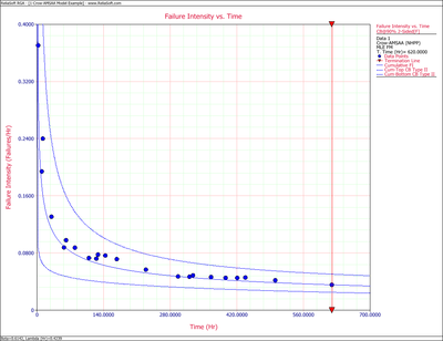
- [math]\displaystyle{ \begin{align} {{\lambda }_{c}}(T)= & 0.03548 \\ {{\lambda }_{i}}(T)= & 0.02179 \end{align}\,\! }[/math]
So, at the 90% confidence level and for [math]\displaystyle{ T=620\,\! }[/math] hours, the Fisher Matrix confidence bounds for the cumulative failure intensity are:
- [math]\displaystyle{ \begin{align} {{[{{\lambda }_{c}}(T)]}_{L}}= & 0.02499 \\ {{[{{\lambda }_{c}}(T)]}_{U}}= & 0.05039 \end{align}\,\! }[/math]
The confidence bounds for the instantaneous failure intensity are:
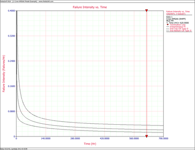
- [math]\displaystyle{ \begin{align} {{[{{\lambda }_{i}}(T)]}_{L}}= & 0.01327 \\ {{[{{\lambda }_{i}}(T)]}_{U}}= & 0.03579 \end{align}\,\! }[/math]
The following figures display plots of the Fisher Matrix confidence bounds for the cumulative and instantaneous failure intensity, respectively.
Crow Bounds
Given that the data is failure terminated, the Crow confidence bounds for the cumulative failure intensity at the 90% confidence level and for [math]\displaystyle{ T=620\,\! }[/math] hours are:
- [math]\displaystyle{ \begin{align} {{[{{\lambda }_{c}}(T)]}_{L}} = & \frac{\chi _{\tfrac{\alpha }{2},2N}^{2}}{2\cdot t} \\ = & \frac{29.787476}{2*620} \\ = & 0.02402 \\ {{[{{\lambda }_{c}}(T)]}_{U}} = & \frac{\chi _{1-\tfrac{\alpha }{2},2N}^{2}}{2\cdot t} \\ = & \frac{60.48089}{2*620} \\ = & 0.048775 \end{align}\,\! }[/math]
The Crow confidence bounds for the instantaneous failure intensity at the 90% confidence level and for [math]\displaystyle{ T=620\,\! }[/math] hours are calculated by first estimating the bounds on the instantaneous MTBF. Once these are calculated, take the inverse as shown below. Details on the confidence bounds for instantaneous MTBF are presented here.
- [math]\displaystyle{ \begin{align} {{[{{\lambda }_{i}}(t)]}_{L}} = & \frac{1}{{{[MTB{{F}_{i}}]}_{U}}} \\ = & \frac{1}{MTB{{F}_{i}}\cdot U} \\ = & 0.01179 \end{align}\,\! }[/math]
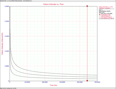
- [math]\displaystyle{ \begin{align} {{[{{\lambda }_{i}}(t)]}_{U}}= & \frac{1}{{{[MTB{{F}_{i}}]}_{L}}} \\ = & \frac{1}{MTB{{F}_{i}}\cdot L} \\ = & 0.03253 \end{align}\,\! }[/math]
The following figures display plots of the Crow confidence bounds for the cumulative and instantaneous failure intensity, respectively.
Failure Times - Example 3
Calculate the confidence bounds on the cumulative and instantaneous MTBF for the data from the example given above.
Solution
Fisher Matrix Bounds
From the previous example:
- [math]\displaystyle{ \begin{align} Var(\hat{\lambda }) = & 0.13519969 \\ Var(\hat{\beta }) = & 0.017105343 \\ Cov(\hat{\beta },\hat{\lambda }) = & -0.046614609 \end{align}\,\! }[/math]
And for [math]\displaystyle{ T=620\,\! }[/math] hours, the partial derivatives of the cumulative and instantaneous MTBF are:
- [math]\displaystyle{ \begin{align} \frac{\partial {{m}_{c}}(T)}{\partial \beta }= & -\frac{1}{\hat{\lambda }}{{T}^{1-\hat{\beta }}}\ln T \\ = & -\frac{1}{0.4239}{{620}^{0.3858}}\ln 620 \\ = & -181.23135 \\ \frac{\partial {{m}_{c}}(T)}{\partial \lambda } = & -\frac{1}{{{\hat{\lambda }}^{2}}}{{T}^{1-\hat{\beta }}} \\ = & -\frac{1}{{{0.4239}^{2}}}{{620}^{0.3858}} \\ = & -66.493299 \\ \frac{\partial {{m}_{i}}(T)}{\partial \beta } = & -\frac{1}{\hat{\lambda }{{\hat{\beta }}^{2}}}{{T}^{1-\beta }}-\frac{1}{\hat{\lambda }\hat{\beta }}{{T}^{1-\hat{\beta }}}\ln T \\ = & -\frac{1}{0.4239\cdot {{0.6142}^{2}}}{{620}^{0.3858}}-\frac{1}{0.4239\cdot 0.6142}{{620}^{0.3858}}\ln 620 \\ = & -369.78634 \\ \frac{\partial {{m}_{i}}(T)}{\partial \lambda } = & -\frac{1}{{{\hat{\lambda }}^{2}}\hat{\beta }}{{T}^{1-\hat{\beta }}} \\ = & -\frac{1}{{{0.4239}^{2}}\cdot 0.6142}\cdot {{620}^{0.3858}} \\ = & -108.26001 \end{align}\,\! }[/math]
Therefore, the variances become:
- [math]\displaystyle{ \begin{align} Var({{\hat{m}}_{c}}(T)) = & {{\left( -181.23135 \right)}^{2}}\cdot 0.017105343+{{\left( -66.493299 \right)}^{2}}\cdot 0.13519969 \\ & -2\cdot \left( -181.23135 \right)\cdot \left( -66.493299 \right)\cdot 0.046614609 \\ = & 36.113376 \end{align}\,\! }[/math]
- [math]\displaystyle{ \begin{align} Var({{\hat{m}}_{i}}(T)) = & {{\left( -369.78634 \right)}^{2}}\cdot 0.017105343+{{\left( -108.26001 \right)}^{2}}\cdot 0.13519969 \\ & -2\cdot \left( -369.78634 \right)\cdot \left( -108.26001 \right)\cdot 0.046614609 \\ = & 191.33709 \end{align}\,\! }[/math]
So, at 90% confidence level and [math]\displaystyle{ T=620\,\! }[/math] hours, the Fisher Matrix confidence bounds are:
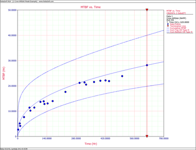
- [math]\displaystyle{ \begin{align} {{[{{m}_{c}}(T)]}_{L}} = & {{{\hat{m}}}_{c}}(t){{e}^{-{{z}_{\alpha }}\sqrt{Var({{{\hat{m}}}_{c}}(t))}/{{{\hat{m}}}_{c}}(t)}} \\ = & 19.84581 \\ {{[{{m}_{c}}(T)]}_{U}} = & {{{\hat{m}}}_{c}}(t){{e}^{{{z}_{\alpha }}\sqrt{Var({{{\hat{m}}}_{c}}(t))}/{{{\hat{m}}}_{c}}(t)}} \\ = & 40.01927 \end{align}\,\! }[/math]
- [math]\displaystyle{ \begin{align} {{[{{m}_{i}}(T)]}_{L}} = & {{{\hat{m}}}_{i}}(t){{e}^{-{{z}_{\alpha }}\sqrt{Var({{{\hat{m}}}_{i}}(t))}/{{{\hat{m}}}_{i}}(t)}} \\ = & 27.94261 \\ {{[{{m}_{i}}(T)]}_{U}} = & {{{\hat{m}}}_{i}}(t){{e}^{{{z}_{\alpha }}\sqrt{Var({{{\hat{m}}}_{i}}(t))}/{{{\hat{m}}}_{i}}(t)}} \\ = & 75.34193 \end{align}\,\! }[/math]
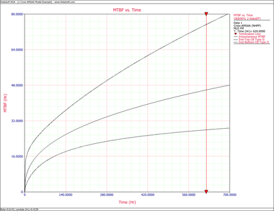
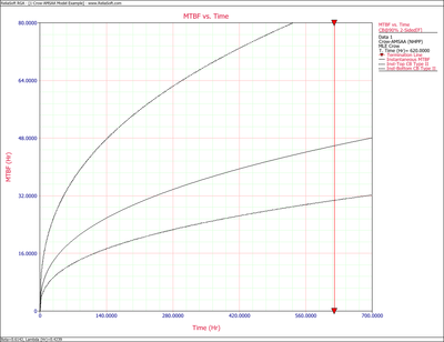
The following two figures show plots of the Fisher Matrix confidence bounds for the cumulative and instantaneous MTBFs.
Crow Bounds
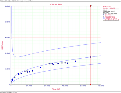
The Crow confidence bounds for the cumulative MTBF and the instantaneous MTBF at the 90% confidence level and for [math]\displaystyle{ T=620\,\! }[/math] hours are:
- [math]\displaystyle{ \begin{align} {{[{{m}_{c}}(T)]}_{L}} = & \frac{1}{{{[{{\lambda }_{c}}(T)]}_{U}}} \\ = & 20.5023 \\ {{[{{m}_{c}}(T)]}_{U}} = & \frac{1}{{{[{{\lambda }_{c}}(T)]}_{L}}} \\ = & 41.6282 \end{align}\,\! }[/math]
- [math]\displaystyle{ \begin{align} {{[MTB{{F}_{i}}]}_{L}} = & MTB{{F}_{i}}\cdot {{\Pi }_{1}} \\ = & 30.7445 \\ {{[MTB{{F}_{i}}]}_{U}} = & MTB{{F}_{i}}\cdot {{\Pi }_{2}} \\ = & 84.7972 \end{align}\,\! }[/math]
The figures below show plots of the Crow confidence bounds for the cumulative and instantaneous MTBF.
Confidence bounds can also be obtained on the parameters [math]\displaystyle{ \hat{\beta }\,\! }[/math] and [math]\displaystyle{ \hat{\lambda }\,\! }[/math]. For Fisher Matrix confidence bounds:
- [math]\displaystyle{ \begin{align} {{\beta }_{L}} = & \hat{\beta }{{e}^{{{z}_{\alpha }}\sqrt{Var(\hat{\beta })}/\hat{\beta }}} \\ = & 0.4325 \\ {{\beta }_{U}} = & \hat{\beta }{{e}^{-{{z}_{\alpha }}\sqrt{Var(\hat{\beta })}/\hat{\beta }}} \\ = & 0.8722 \end{align}\,\! }[/math]
and:
- [math]\displaystyle{ \begin{align} {{\lambda }_{L}} = & \hat{\lambda }{{e}^{{{z}_{\alpha }}\sqrt{Var(\hat{\lambda })}/\hat{\lambda }}} \\ = & 0.1016 \\ {{\lambda }_{U}} = & \hat{\lambda }{{e}^{-{{z}_{\alpha }}\sqrt{Var(\hat{\lambda })}/\hat{\lambda }}} \\ = & 1.7691 \end{align}\,\! }[/math]
For Crow confidence bounds:
- [math]\displaystyle{ \begin{align} {{\beta }_{L}}= & 0.4527 \\ {{\beta }_{U}}= & 0.9350 \end{align}\,\! }[/math]
and:
- [math]\displaystyle{ \begin{align} {{\lambda }_{L}}= & 0.2870 \\ {{\lambda }_{U}}= & 0.5827 \end{align}\,\! }[/math]

