Crow-AMSAA Model Examples
 |
New format available! This reference is now available in a new format that offers faster page load, improved display for calculations and images and more targeted search.
As of January 2024, this Reliawiki page will not continue to be updated. Please update all links and bookmarks to the latest references at RGA examples and RGA reference examples.
These examples appear in the Reliability Growth and Repairable System Analysis Reference book.
Failure Times Model
A prototype of a system was tested with design changes incorporated during the test. The following table presents the data collected over the entire test. Find the Crow-AMSAA parameters and the intensity function using maximum likelihood estimators.
| Row | Time to Event (hr) | [math]\displaystyle{ ln{(T)}\,\! }[/math] |
|---|---|---|
| 1 | 2.7 | 0.99325 |
| 2 | 10.3 | 2.33214 |
| 3 | 12.5 | 2.52573 |
| 4 | 30.6 | 3.42100 |
| 5 | 57.0 | 4.04305 |
| 6 | 61.3 | 4.11578 |
| 7 | 80.0 | 4.38203 |
| 8 | 109.5 | 4.69592 |
| 9 | 125.0 | 4.82831 |
| 10 | 128.6 | 4.85671 |
| 11 | 143.8 | 4.96842 |
| 12 | 167.9 | 5.12337 |
| 13 | 229.2 | 5.43459 |
| 14 | 296.7 | 5.69272 |
| 15 | 320.6 | 5.77019 |
| 16 | 328.2 | 5.79362 |
| 17 | 366.2 | 5.90318 |
| 18 | 396.7 | 5.98318 |
| 19 | 421.1 | 6.04287 |
| 20 | 438.2 | 6.08268 |
| 21 | 501.2 | 6.21701 |
| 22 | 620.0 | 6.42972 |
Solution
For the failure terminated test, [math]\displaystyle{ {\beta}\,\! }[/math] is:
- [math]\displaystyle{ \begin{align} \widehat{\beta }&=\frac{n}{n\ln {{T}^{*}}-\underset{i=1}{\overset{n}{\mathop{\sum }}}\,\ln {{T}_{i}}} \\ &=\frac{22}{22\ln 620-\underset{i=1}{\overset{22}{\mathop{\sum }}}\,\ln {{T}_{i}}} \\ \end{align}\,\! }[/math]
where:
- [math]\displaystyle{ \underset{i=1}{\overset{22}{\mathop \sum }}\,\ln {{T}_{i}}=105.6355\,\! }[/math]
Then:
- [math]\displaystyle{ \widehat{\beta }=\frac{22}{22\ln 620-105.6355}=0.6142\,\! }[/math]
And for [math]\displaystyle{ {\lambda}\,\! }[/math] :
- [math]\displaystyle{ \begin{align} \widehat{\lambda }&=\frac{n}{{{T}^{*\beta }}} \\ & =\frac{22}{{{620}^{0.6142}}}=0.4239 \\ \end{align}\,\! }[/math]
Therefore, [math]\displaystyle{ {{\lambda }_{i}}(T)\,\! }[/math] becomes:
- [math]\displaystyle{ \begin{align} {{\widehat{\lambda }}_{i}}(T)= & 0.4239\cdot 0.6142\cdot {{620}^{-0.3858}} \\ = & 0.0217906\frac{\text{failures}}{\text{hr}} \end{align}\,\! }[/math]
The next figure shows the plot of the failure rate. If no further changes are made, the estimated MTBF is [math]\displaystyle{ \tfrac{1}{0.0217906}\,\! }[/math] or 46 hours.

Confidence Bounds
Example - Confidence Bounds on Failure Intensity
Using the values of [math]\displaystyle{ \hat{\beta }\,\! }[/math] and [math]\displaystyle{ \hat{\lambda }\,\! }[/math] estimated in the example given above, calculate the 90% 2-sided confidence bounds on the cumulative and instantaneous failure intensity.
Solution
Fisher Matrix Bounds
The partial derivatives for the Fisher Matrix confidence bounds are:
- [math]\displaystyle{ \begin{align} \frac{{{\partial }^{2}}\Lambda }{\partial {{\lambda }^{2}}} = & -\frac{22}{{{0.4239}^{2}}}=-122.43 \\ \frac{{{\partial }^{2}}\Lambda }{\partial {{\beta }^{2}}} = & -\frac{22}{{{0.6142}^{2}}}-0.4239\cdot {{620}^{0.6142}}{{(\ln 620)}^{2}}=-967.68 \\ \frac{{{\partial }^{2}}\Lambda }{\partial \lambda \partial \beta } = & -{{620}^{0.6142}}\ln 620=-333.64 \end{align}\,\! }[/math]
The Fisher Matrix then becomes:
- [math]\displaystyle{ \begin{align} \begin{bmatrix}122.43 & 333.64\\ 333.64 & 967.68\end{bmatrix}^{-1} & = \begin{bmatrix}Var(\hat{\lambda}) & Cov(\hat{\beta},\hat{\lambda})\\ Cov(\hat{\beta},\hat{\lambda}) & Var(\hat{\beta})\end{bmatrix} \\ & = \begin{bmatrix} 0.13519969 & -0.046614609\\ -0.046614609 & 0.017105343 \end{bmatrix} \end{align}\,\! }[/math]
For [math]\displaystyle{ T=620\,\! }[/math] hours, the partial derivatives of the cumulative and instantaneous failure intensities are:
- [math]\displaystyle{ \begin{align} \frac{\partial {{\lambda }_{c}}(T)}{\partial \beta }= & \hat{\lambda }{{T}^{\hat{\beta }-1}}\ln (T) \\ = & 0.4239\cdot {{620}^{-0.3858}}\ln 620 \\ = & 0.22811336 \\ \frac{\partial {{\lambda }_{c}}(T)}{\partial \lambda }= & {{T}^{\hat{\beta }-1}} \\ = & {{620}^{-0.3858}} \\ = & 0.083694185 \end{align}\,\! }[/math]
- [math]\displaystyle{ \begin{align} \frac{\partial {{\lambda }_{i}}(T)}{\partial \beta }= & \hat{\lambda }{{T}^{\hat{\beta }-1}}+\hat{\lambda }\hat{\beta }{{T}^{\hat{\beta }-1}}\ln T \\ = & 0.4239\cdot {{620}^{-0.3858}}+0.4239\cdot 0.6142\cdot {{620}^{-0.3858}}\ln 620 \\ = & 0.17558519 \end{align}\,\! }[/math]
- [math]\displaystyle{ \begin{align} \frac{\partial {{\lambda }_{i}}(T)}{\partial \lambda }= & \hat{\beta }{{T}^{\hat{\beta }-1}} \\ = & 0.6142\cdot {{620}^{-0.3858}} \\ = & 0.051404969 \end{align}\,\! }[/math]
Therefore, the variances become:
- [math]\displaystyle{ \begin{align} Var(\hat{\lambda_{c}}(T)) & = 0.22811336^{2}\cdot 0.017105343\ + 0.083694185^{2} \cdot 0.13519969\ -2\cdot 0.22811336\cdot 0.083694185\cdot 0.046614609 \\ & = 0.00005721408 \\ Var(\hat{\lambda_{i}}(T)) & = 0.17558519^{2}\cdot 0.01715343\ + 0.051404969^{2}\cdot 0.13519969\ -2\cdot 0.17558519\cdot 0.051404969\cdot 0.046614609 \\ &= 0.0000431393 \end{align}\,\! }[/math]
The cumulative and instantaneous failure intensities at [math]\displaystyle{ T=620\,\! }[/math] hours are:
- [math]\displaystyle{ \begin{align} {{\lambda }_{c}}(T)= & 0.03548 \\ {{\lambda }_{i}}(T)= & 0.02179 \end{align}\,\! }[/math]
So, at the 90% confidence level and for [math]\displaystyle{ T=620\,\! }[/math] hours, the Fisher Matrix confidence bounds for the cumulative failure intensity are:
- [math]\displaystyle{ \begin{align} {{[{{\lambda }_{c}}(T)]}_{L}}= & 0.02499 \\ {{[{{\lambda }_{c}}(T)]}_{U}}= & 0.05039 \end{align}\,\! }[/math]
The confidence bounds for the instantaneous failure intensity are:
- [math]\displaystyle{ \begin{align} {{[{{\lambda }_{i}}(T)]}_{L}}= & 0.01327 \\ {{[{{\lambda }_{i}}(T)]}_{U}}= & 0.03579 \end{align}\,\! }[/math]
The following figures display plots of the Fisher Matrix confidence bounds for the cumulative and instantaneous failure intensity, respectively.


Crow Bounds
Given that the data is failure terminated, the Crow confidence bounds for the cumulative failure intensity at the 90% confidence level and for [math]\displaystyle{ T=620\,\! }[/math] hours are:
- [math]\displaystyle{ \begin{align} {{[{{\lambda }_{c}}(T)]}_{L}} = & \frac{\chi _{\tfrac{\alpha }{2},2N}^{2}}{2\cdot t} \\ = & \frac{29.787476}{2*620} \\ = & 0.02402 \\ {{[{{\lambda }_{c}}(T)]}_{U}} = & \frac{\chi _{1-\tfrac{\alpha }{2},2N}^{2}}{2\cdot t} \\ = & \frac{60.48089}{2*620} \\ = & 0.048775 \end{align}\,\! }[/math]
The Crow confidence bounds for the instantaneous failure intensity at the 90% confidence level and for [math]\displaystyle{ T=620\,\! }[/math] hours are calculated by first estimating the bounds on the instantaneous MTBF. Once these are calculated, take the inverse as shown below. Details on the confidence bounds for instantaneous MTBF are presented here.
- [math]\displaystyle{ \begin{align} {{[{{\lambda }_{i}}(t)]}_{L}} = & \frac{1}{{{[MTB{{F}_{i}}]}_{U}}} \\ = & \frac{1}{MTB{{F}_{i}}\cdot U} \\ = & 0.01179 \end{align}\,\! }[/math]
- [math]\displaystyle{ \begin{align} {{[{{\lambda }_{i}}(t)]}_{U}}= & \frac{1}{{{[MTB{{F}_{i}}]}_{L}}} \\ = & \frac{1}{MTB{{F}_{i}}\cdot L} \\ = & 0.03253 \end{align}\,\! }[/math]
The following figures display plots of the Crow confidence bounds for the cumulative and instantaneous failure intensity, respectively.


Example - Confidence Bounds on MTBF
Calculate the confidence bounds on the cumulative and instantaneous MTBF for the data from the example given above.
Solution
Fisher Matrix Bounds
From the previous example:
- [math]\displaystyle{ \begin{align} Var(\hat{\lambda }) = & 0.13519969 \\ Var(\hat{\beta }) = & 0.017105343 \\ Cov(\hat{\beta },\hat{\lambda }) = & -0.046614609 \end{align}\,\! }[/math]
And for [math]\displaystyle{ T=620\,\! }[/math] hours, the partial derivatives of the cumulative and instantaneous MTBF are:
- [math]\displaystyle{ \begin{align} \frac{\partial {{m}_{c}}(T)}{\partial \beta }= & -\frac{1}{\hat{\lambda }}{{T}^{1-\hat{\beta }}}\ln T \\ = & -\frac{1}{0.4239}{{620}^{0.3858}}\ln 620 \\ = & -181.23135 \\ \frac{\partial {{m}_{c}}(T)}{\partial \lambda } = & -\frac{1}{{{\hat{\lambda }}^{2}}}{{T}^{1-\hat{\beta }}} \\ = & -\frac{1}{{{0.4239}^{2}}}{{620}^{0.3858}} \\ = & -66.493299 \\ \frac{\partial {{m}_{i}}(T)}{\partial \beta } = & -\frac{1}{\hat{\lambda }{{\hat{\beta }}^{2}}}{{T}^{1-\beta }}-\frac{1}{\hat{\lambda }\hat{\beta }}{{T}^{1-\hat{\beta }}}\ln T \\ = & -\frac{1}{0.4239\cdot {{0.6142}^{2}}}{{620}^{0.3858}}-\frac{1}{0.4239\cdot 0.6142}{{620}^{0.3858}}\ln 620 \\ = & -369.78634 \\ \frac{\partial {{m}_{i}}(T)}{\partial \lambda } = & -\frac{1}{{{\hat{\lambda }}^{2}}\hat{\beta }}{{T}^{1-\hat{\beta }}} \\ = & -\frac{1}{{{0.4239}^{2}}\cdot 0.6142}\cdot {{620}^{0.3858}} \\ = & -108.26001 \end{align}\,\! }[/math]
Therefore, the variances become:
- [math]\displaystyle{ \begin{align} Var({{\hat{m}}_{c}}(T)) = & {{\left( -181.23135 \right)}^{2}}\cdot 0.017105343+{{\left( -66.493299 \right)}^{2}}\cdot 0.13519969 \\ & -2\cdot \left( -181.23135 \right)\cdot \left( -66.493299 \right)\cdot 0.046614609 \\ = & 36.113376 \end{align}\,\! }[/math]
- [math]\displaystyle{ \begin{align} Var({{\hat{m}}_{i}}(T)) = & {{\left( -369.78634 \right)}^{2}}\cdot 0.017105343+{{\left( -108.26001 \right)}^{2}}\cdot 0.13519969 \\ & -2\cdot \left( -369.78634 \right)\cdot \left( -108.26001 \right)\cdot 0.046614609 \\ = & 191.33709 \end{align}\,\! }[/math]
So, at 90% confidence level and [math]\displaystyle{ T=620\,\! }[/math] hours, the Fisher Matrix confidence bounds are:
- [math]\displaystyle{ \begin{align} {{[{{m}_{c}}(T)]}_{L}} = & {{{\hat{m}}}_{c}}(t){{e}^{-{{z}_{\alpha }}\sqrt{Var({{{\hat{m}}}_{c}}(t))}/{{{\hat{m}}}_{c}}(t)}} \\ = & 19.84581 \\ {{[{{m}_{c}}(T)]}_{U}} = & {{{\hat{m}}}_{c}}(t){{e}^{{{z}_{\alpha }}\sqrt{Var({{{\hat{m}}}_{c}}(t))}/{{{\hat{m}}}_{c}}(t)}} \\ = & 40.01927 \end{align}\,\! }[/math]
- [math]\displaystyle{ \begin{align} {{[{{m}_{i}}(T)]}_{L}} = & {{{\hat{m}}}_{i}}(t){{e}^{-{{z}_{\alpha }}\sqrt{Var({{{\hat{m}}}_{i}}(t))}/{{{\hat{m}}}_{i}}(t)}} \\ = & 27.94261 \\ {{[{{m}_{i}}(T)]}_{U}} = & {{{\hat{m}}}_{i}}(t){{e}^{{{z}_{\alpha }}\sqrt{Var({{{\hat{m}}}_{i}}(t))}/{{{\hat{m}}}_{i}}(t)}} \\ = & 75.34193 \end{align}\,\! }[/math]
The following two figures show plots of the Fisher Matrix confidence bounds for the cumulative and instantaneous MTBFs.


Crow Bounds
The Crow confidence bounds for the cumulative MTBF and the instantaneous MTBF at the 90% confidence level and for [math]\displaystyle{ T=620\,\! }[/math] hours are:
- [math]\displaystyle{ \begin{align} {{[{{m}_{c}}(T)]}_{L}} = & \frac{1}{{{[{{\lambda }_{c}}(T)]}_{U}}} \\ = & 20.5023 \\ {{[{{m}_{c}}(T)]}_{U}} = & \frac{1}{{{[{{\lambda }_{c}}(T)]}_{L}}} \\ = & 41.6282 \end{align}\,\! }[/math]
- [math]\displaystyle{ \begin{align} {{[MTB{{F}_{i}}]}_{L}} = & MTB{{F}_{i}}\cdot {{\Pi }_{1}} \\ = & 30.7445 \\ {{[MTB{{F}_{i}}]}_{U}} = & MTB{{F}_{i}}\cdot {{\Pi }_{2}} \\ = & 84.7972 \end{align}\,\! }[/math]
The figures below show plots of the Crow confidence bounds for the cumulative and instantaneous MTBF.


Confidence bounds can also be obtained on the parameters [math]\displaystyle{ \hat{\beta }\,\! }[/math] and [math]\displaystyle{ \hat{\lambda }\,\! }[/math]. For Fisher Matrix confidence bounds:
- [math]\displaystyle{ \begin{align} {{\beta }_{L}} = & \hat{\beta }{{e}^{{{z}_{\alpha }}\sqrt{Var(\hat{\beta })}/\hat{\beta }}} \\ = & 0.4325 \\ {{\beta }_{U}} = & \hat{\beta }{{e}^{-{{z}_{\alpha }}\sqrt{Var(\hat{\beta })}/\hat{\beta }}} \\ = & 0.8722 \end{align}\,\! }[/math]
and:
- [math]\displaystyle{ \begin{align} {{\lambda }_{L}} = & \hat{\lambda }{{e}^{{{z}_{\alpha }}\sqrt{Var(\hat{\lambda })}/\hat{\lambda }}} \\ = & 0.1016 \\ {{\lambda }_{U}} = & \hat{\lambda }{{e}^{-{{z}_{\alpha }}\sqrt{Var(\hat{\lambda })}/\hat{\lambda }}} \\ = & 1.7691 \end{align}\,\! }[/math]
For Crow confidence bounds:
- [math]\displaystyle{ \begin{align} {{\beta }_{L}}= & 0.4527 \\ {{\beta }_{U}}= & 0.9350 \end{align}\,\! }[/math]
and:
- [math]\displaystyle{ \begin{align} {{\lambda }_{L}}= & 0.2870 \\ {{\lambda }_{U}}= & 0.5827 \end{align}\,\! }[/math]
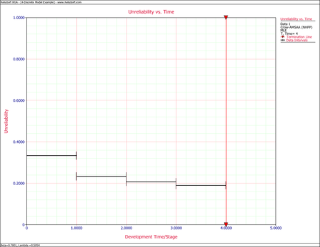
Discrete Model
A one-shot system underwent reliability growth development testing for a total of 68 trials. Delayed corrective actions were incorporated after the 14th, 33rd and 48th trials. From trial 49 to trial 68, the configuration was not changed.
- Configuration 1 experienced 5 failures,
- Configuration 2 experienced 3 failures,
- Configuration 3 experienced 4 failures and
- Configuration 4 experienced 4 failures.
Do the following:
- Estimate the parameters of the Crow-AMSAA model using maximum likelihood estimation.
- Estimate the unreliability and reliability by configuration.
Solution
- The parameter estimates for the Crow-AMSAA model using the parameter estimation for discrete data methodology yields [math]\displaystyle{ \lambda = 0.5954\,\! }[/math] and [math]\displaystyle{ \beta =0.7801\,\! }[/math].
- The following table displays the results for probability of failure and reliability, and these results are displayed in the next two plots.
Estimated Failure Probability and Reliability by Configuration Configuration([math]\displaystyle{ i\,\! }[/math]) Estimated Failure Probability Estimated Reliability 1 0.333 0.667 2 0.234 0.766 3 0.206 0.794 4 0.190 0.810