Crow Extended Confidence Bounds Example 2: Difference between revisions
Kate Racaza (talk | contribs) No edit summary |
Lisa Hacker (talk | contribs) No edit summary |
||
| (5 intermediate revisions by 2 users not shown) | |||
| Line 1: | Line 1: | ||
<noinclude>{{Banner RGA Examples}} | <noinclude>{{Banner RGA Examples}} | ||
''This example appears in the [ | ''This example appears in the [https://help.reliasoft.com/reference/reliability_growth_and_repairable_system_analysis Reliability growth reference]''. | ||
</noinclude> | </noinclude> | ||
| Line 10: | Line 10: | ||
For this example, there are A, BC and BD failure modes, so the estimated demonstrated failure intensity, <math>{{\hat{\lambda }}_{D}}(T)\,\!</math>, is simply the Crow-AMSAA model applied to all A, BC, and BD data. | For this example, there are A, BC and BD failure modes, so the estimated demonstrated failure intensity, <math>{{\hat{\lambda }}_{D}}(T)\,\!</math>, is simply the Crow-AMSAA model applied to all A, BC, and BD data. | ||
:<math>{{\hat{\lambda }}_{D}}(T)={{\widehat{\lambda }}_{CA}}=\widehat{\lambda }\widehat{\beta }{{T}^{\widehat{\beta }-1}}=0.12744\,\!</math> | |||
Therefore, the demonstrated MTBF is: | Therefore, the demonstrated MTBF is: | ||
:<math>MTB{{F}_{D}}={{[{{\hat{\lambda }}_{D}}(T)]}^{-1}}=7.84708\,\!</math> | |||
Based on this value, the Fisher Matrix confidence bounds for the demonstrated failure intensity at the 90% confidence level are: | Based on this value, the Fisher Matrix confidence bounds for the demonstrated failure intensity at the 90% confidence level are: | ||
:<math>\begin{align} | |||
{{[{{\lambda }_{D}}(T)]}_{L}} = & {{{\hat{\lambda }}}_{CA}}(T){{e}^{{{z}_{\alpha }}\sqrt{Var({{{\hat{\lambda }}}_{CA}}(T))}/{{{\hat{\lambda }}}_{ | {{[{{\lambda }_{D}}(T)]}_{L}} = & {{{\hat{\lambda }}}_{CA}}(T){{e}^{{{z}_{\alpha }}\sqrt{Var({{{\hat{\lambda }}}_{CA}}(T))}/{{{\hat{\lambda }}}_{CA}}(T)}} \\ | ||
= & 0.09339 | = & 0.09339 | ||
\end{align}\,\!</math> | \end{align}\,\!</math> | ||
:<math>\begin{align} | |||
{{[{{\lambda }_{D}}(T)]}_{U}} = & {{{\hat{\lambda }}}_{CA}}(T){{e}^{-{{z}_{\alpha }}\sqrt{Var({{{\hat{\lambda }}}_{CA}}(T))}/{{{\hat{\lambda }}}_{CA}}(T)}} \\ | |||
{{[{{\lambda }_{D}}(T)]}_{U}} = & {{{\hat{\lambda }}}_{CA}}(T){{e}^{-{{z}_{\alpha }}\sqrt{Var({{{\hat{\lambda }}}_{CA}}(T))}/{{{\hat{\lambda }}}_{ | |||
= & 0.17390 | = & 0.17390 | ||
\end{align}\,\!</math> | \end{align}\,\!</math> | ||
The Fisher Matrix confidence bounds for the demonstrated MTBF at the 90% confidence level are: | The Fisher Matrix confidence bounds for the demonstrated MTBF at the 90% confidence level are: | ||
:<math>\begin{align} | |||
MTB{{F}_{{{D}_{L}}}} = & \frac{1}{{{[{{\lambda }_{D}}(T)]}_{U}}} \\ | MTB{{F}_{{{D}_{L}}}} = & \frac{1}{{{[{{\lambda }_{D}}(T)]}_{U}}} \\ | ||
= & 5.75054 \\ | = & 5.75054 \\ | ||
| Line 40: | Line 36: | ||
= & 10.70799 | = & 10.70799 | ||
\end{align}\,\!</math> | \end{align}\,\!</math> | ||
The Crow confidence bounds for the demonstrated MTBF at the 90% confidence level are: | The Crow confidence bounds for the demonstrated MTBF at the 90% confidence level are: | ||
:<math>\begin{align} | |||
MTB{{F}_{{{D}_{L}}}} = & \frac{1}{{{[{{\lambda }_{D}}(T)]}_{U}}} \\ | MTB{{F}_{{{D}_{L}}}} = & \frac{1}{{{[{{\lambda }_{D}}(T)]}_{U}}} \\ | ||
= & \frac{1}{{{\widehat{\lambda }}_{D}}(T)\tfrac{{{\chi }^{2}}(2N,\alpha /2)}{2N}} \\ | = & \frac{1}{{{\widehat{\lambda }}_{D}}(T)\tfrac{{{\chi }^{2}}(2N,\alpha /2)}{2N}} \\ | ||
| Line 52: | Line 47: | ||
= & 10.8779 | = & 10.8779 | ||
\end{align}\,\!</math> | \end{align}\,\!</math> | ||
The projected failure intensity is: | The projected failure intensity is: | ||
:<math>\begin{align} | |||
\hat{\lambda}_P (T) &= \widehat{\lambda}_{CA} - \widehat{\lambda}_{BD} + \sum_{i=1}^M (1-d_i) \tfrac{N_i}{T} + \bar{d}\widehat{h}(T|BD) \\ | \hat{\lambda}_P (T) &= \widehat{\lambda}_{CA} - \widehat{\lambda}_{BD} + \sum_{i=1}^M (1-d_i) \tfrac{N_i}{T} + \bar{d}\widehat{h}(T|BD) \\ | ||
&= 0.0885 \,\! | &= 0.0885 \,\! | ||
\end{align}</math> | \end{align}</math> | ||
Based on this value, the Fisher Matrix confidence bounds at the 90% confidence level for the projected failure intensity are: | Based on this value, the Fisher Matrix confidence bounds at the 90% confidence level for the projected failure intensity are: | ||
:<math>\begin{align} | |||
{{[{{\lambda }_{P}}(T)]}_{L}} = & {{{\hat{\lambda }}}_{P}}(T){{e}^{{{z}_{\alpha }}\sqrt{Var({{{\hat{\lambda }}}_{P}}(T))}/{{{\hat{\lambda }}}_{P}}(T)}} \\ | {{[{{\lambda }_{P}}(T)]}_{L}} = & {{{\hat{\lambda }}}_{P}}(T){{e}^{{{z}_{\alpha }}\sqrt{Var({{{\hat{\lambda }}}_{P}}(T))}/{{{\hat{\lambda }}}_{P}}(T)}} \\ | ||
= & 0.0681 | = & 0.0681 | ||
\end{align}\,\!</math> | \end{align}\,\!</math> | ||
:<math>\begin{align} | |||
{{[{{\lambda }_{P}}(T)]}_{U}} = & {{{\hat{\lambda }}}_{P}}(T){{e}^{-{{z}_{\alpha }}\sqrt{Var({{{\hat{\lambda }}}_{P}}(T))}/{{{\hat{\lambda }}}_{P}}(T)}} \\ | {{[{{\lambda }_{P}}(T)]}_{U}} = & {{{\hat{\lambda }}}_{P}}(T){{e}^{-{{z}_{\alpha }}\sqrt{Var({{{\hat{\lambda }}}_{P}}(T))}/{{{\hat{\lambda }}}_{P}}(T)}} \\ | ||
= & 0.1152 | = & 0.1152 | ||
\end{align}\,\!</math> | \end{align}\,\!</math> | ||
The Fisher Matrix confidence bounds for the projected MTBF at the 90% confidence level are: | The Fisher Matrix confidence bounds for the projected MTBF at the 90% confidence level are: | ||
:<math>\begin{align} | |||
MTB{{F}_{{{P}_{L}}}} = & \frac{1}{{{[{{\lambda }_{P}}(T)]}_{U}}} \\ | MTB{{F}_{{{P}_{L}}}} = & \frac{1}{{{[{{\lambda }_{P}}(T)]}_{U}}} \\ | ||
= & 8.6818 \\ | = & 8.6818 \\ | ||
| Line 84: | Line 75: | ||
= & 14.6926 | = & 14.6926 | ||
\end{align}\,\!</math> | \end{align}\,\!</math> | ||
The Crow confidence bounds for the projected failure intensity are: | The Crow confidence bounds for the projected failure intensity are: | ||
:<math>\begin{align} | |||
{{[{{\lambda }_{P}}(T)]}_{L}} = & {{{\hat{\lambda }}}_{P}}(T)+\frac{{{C}^{2}}}{2}-\sqrt{{{{\hat{\lambda }}}_{P}}(T)\cdot \ \,{{C}^{2}}+\frac{{{C}^{4}}}{4}} \\ | {{[{{\lambda }_{P}}(T)]}_{L}} = & {{{\hat{\lambda }}}_{P}}(T)+\frac{{{C}^{2}}}{2}-\sqrt{{{{\hat{\lambda }}}_{P}}(T)\cdot \ \,{{C}^{2}}+\frac{{{C}^{4}}}{4}} \\ | ||
= & 0.0672 \\ | = & 0.0672 \\ | ||
| Line 94: | Line 84: | ||
= & 0.1166 | = & 0.1166 | ||
\end{align}\,\!</math> | \end{align}\,\!</math> | ||
The Crow confidence bounds for the projected MTBF at the 90% confidence level are: | The Crow confidence bounds for the projected MTBF at the 90% confidence level are: | ||
:<math>\begin{align} | |||
MTB{{F}_{{{P}_{L}}}} = & \frac{1}{{{[{{\widehat{\lambda }}_{P}}(T)]}_{U}}} \\ | MTB{{F}_{{{P}_{L}}}} = & \frac{1}{{{[{{\widehat{\lambda }}_{P}}(T)]}_{U}}} \\ | ||
= & 8.5743 \\ | = & 8.5743 \\ | ||
| Line 104: | Line 93: | ||
= & 14.8769 | = & 14.8769 | ||
\end{align}\,\!</math> | \end{align}\,\!</math> | ||
The growth potential failure intensity is: | The growth potential failure intensity is: | ||
:<math>\widehat{\lambda}_{GP} = \widehat{\lambda}_{CA} - \widehat{\lambda}_{BD} + \sum_{i=1}^M (1-d_i) \tfrac{N_i}{T} = 0.0670 \,\!</math> | |||
Based on this value, the Fisher Matrix and Crow confidence bounds at the 90% confidence level for the growth potential failure intensity are: | Based on this value, the Fisher Matrix and Crow confidence bounds at the 90% confidence level for the growth potential failure intensity are: | ||
:<math>\begin{align} | |||
{{r}_{L}} = & {{{\hat{r}}}_{GP}}+\frac{{{C}^{2}}}{2}-\sqrt{{{{\hat{r}}}_{GP}}{{C}^{2}}+\frac{{{C}^{4}}}{4}} \\ | {{r}_{L}} = & {{{\hat{r}}}_{GP}}+\frac{{{C}^{2}}}{2}-\sqrt{{{{\hat{r}}}_{GP}}{{C}^{2}}+\frac{{{C}^{4}}}{4}} \\ | ||
= & 0.0488 \\ | = & 0.0488 \\ | ||
| Line 120: | Line 106: | ||
= & 0.0919 | = & 0.0919 | ||
\end{align}\,\!</math> | \end{align}\,\!</math> | ||
The Fisher Matrix and Crow confidence bounds for the growth potential MTBF at the 90% confidence level are: | The Fisher Matrix and Crow confidence bounds for the growth potential MTBF at the 90% confidence level are: | ||
:<math>\begin{align} | |||
MTB{{F}_{G{{P}_{L}}}} = & \frac{1}{{{r}_{U}}} \\ | MTB{{F}_{G{{P}_{L}}}} = & \frac{1}{{{r}_{U}}} \\ | ||
= & 10.8790 \\ | = & 10.8790 \\ | ||
| Line 130: | Line 115: | ||
= & 20.4855 | = & 20.4855 | ||
\end{align}\,\!</math> | \end{align}\,\!</math> | ||
The figure below shows the Fisher Matrix confidence bounds at the 90% confidence level for the demonstrated, projected and growth potential MTBF. | The figure below shows the Fisher Matrix confidence bounds at the 90% confidence level for the demonstrated, projected and growth potential MTBF. | ||
[[Image:rga9.10.png|center| | [[Image:rga9.10.png|center|450px]] | ||
The next figure shows these bounds based on the Crow method. | The next figure shows these bounds based on the Crow method. | ||
[[Image:rga9.11.png|center| | [[Image:rga9.11.png|center|450px]] | ||
Latest revision as of 21:31, 18 September 2023
New format available! This reference is now available in a new format that offers faster page load, improved display for calculations and images and more targeted search.
As of January 2024, this Reliawiki page will not continue to be updated. Please update all links and bookmarks to the latest references at RGA examples and RGA reference examples.
This example appears in the Reliability growth reference.
Calculate the 2-sided confidence bounds at the 90% confidence level on the demonstrated, projected and growth potential MTBF for the Test-Fix-Find-Test data in the Crow Extended Test-Fix-Find-Test Example.
Solution
For this example, there are A, BC and BD failure modes, so the estimated demonstrated failure intensity, [math]\displaystyle{ {{\hat{\lambda }}_{D}}(T)\,\! }[/math], is simply the Crow-AMSAA model applied to all A, BC, and BD data.
- [math]\displaystyle{ {{\hat{\lambda }}_{D}}(T)={{\widehat{\lambda }}_{CA}}=\widehat{\lambda }\widehat{\beta }{{T}^{\widehat{\beta }-1}}=0.12744\,\! }[/math]
Therefore, the demonstrated MTBF is:
- [math]\displaystyle{ MTB{{F}_{D}}={{[{{\hat{\lambda }}_{D}}(T)]}^{-1}}=7.84708\,\! }[/math]
Based on this value, the Fisher Matrix confidence bounds for the demonstrated failure intensity at the 90% confidence level are:
- [math]\displaystyle{ \begin{align} {{[{{\lambda }_{D}}(T)]}_{L}} = & {{{\hat{\lambda }}}_{CA}}(T){{e}^{{{z}_{\alpha }}\sqrt{Var({{{\hat{\lambda }}}_{CA}}(T))}/{{{\hat{\lambda }}}_{CA}}(T)}} \\ = & 0.09339 \end{align}\,\! }[/math]
- [math]\displaystyle{ \begin{align} {{[{{\lambda }_{D}}(T)]}_{U}} = & {{{\hat{\lambda }}}_{CA}}(T){{e}^{-{{z}_{\alpha }}\sqrt{Var({{{\hat{\lambda }}}_{CA}}(T))}/{{{\hat{\lambda }}}_{CA}}(T)}} \\ = & 0.17390 \end{align}\,\! }[/math]
The Fisher Matrix confidence bounds for the demonstrated MTBF at the 90% confidence level are:
- [math]\displaystyle{ \begin{align} MTB{{F}_{{{D}_{L}}}} = & \frac{1}{{{[{{\lambda }_{D}}(T)]}_{U}}} \\ = & 5.75054 \\ MTB{{F}_{{{D}_{U}}}} = & \frac{1}{{{[{{\lambda }_{D}}(T)]}_{L}}} \\ = & 10.70799 \end{align}\,\! }[/math]
The Crow confidence bounds for the demonstrated MTBF at the 90% confidence level are:
- [math]\displaystyle{ \begin{align} MTB{{F}_{{{D}_{L}}}} = & \frac{1}{{{[{{\lambda }_{D}}(T)]}_{U}}} \\ = & \frac{1}{{{\widehat{\lambda }}_{D}}(T)\tfrac{{{\chi }^{2}}(2N,\alpha /2)}{2N}} \\ = & 5.6325 \\ MTB{{F}_{{{D}_{U}}}} = & \frac{1}{{{[{{\lambda }_{D}}(T)]}_{L}}} \\ = & \frac{1}{{{\widehat{\lambda }}_{D}}(T)\tfrac{{{\chi }^{2}}(2N,1-\alpha /2)}{2N}} \\ = & 10.8779 \end{align}\,\! }[/math]
The projected failure intensity is:
- [math]\displaystyle{ \begin{align} \hat{\lambda}_P (T) &= \widehat{\lambda}_{CA} - \widehat{\lambda}_{BD} + \sum_{i=1}^M (1-d_i) \tfrac{N_i}{T} + \bar{d}\widehat{h}(T|BD) \\ &= 0.0885 \,\! \end{align} }[/math]
Based on this value, the Fisher Matrix confidence bounds at the 90% confidence level for the projected failure intensity are:
- [math]\displaystyle{ \begin{align} {{[{{\lambda }_{P}}(T)]}_{L}} = & {{{\hat{\lambda }}}_{P}}(T){{e}^{{{z}_{\alpha }}\sqrt{Var({{{\hat{\lambda }}}_{P}}(T))}/{{{\hat{\lambda }}}_{P}}(T)}} \\ = & 0.0681 \end{align}\,\! }[/math]
- [math]\displaystyle{ \begin{align} {{[{{\lambda }_{P}}(T)]}_{U}} = & {{{\hat{\lambda }}}_{P}}(T){{e}^{-{{z}_{\alpha }}\sqrt{Var({{{\hat{\lambda }}}_{P}}(T))}/{{{\hat{\lambda }}}_{P}}(T)}} \\ = & 0.1152 \end{align}\,\! }[/math]
The Fisher Matrix confidence bounds for the projected MTBF at the 90% confidence level are:
- [math]\displaystyle{ \begin{align} MTB{{F}_{{{P}_{L}}}} = & \frac{1}{{{[{{\lambda }_{P}}(T)]}_{U}}} \\ = & 8.6818 \\ MTB{{F}_{{{P}_{U}}}} = & \frac{1}{{{[{{\lambda }_{P}}(T)]}_{L}}} \\ = & 14.6926 \end{align}\,\! }[/math]
The Crow confidence bounds for the projected failure intensity are:
- [math]\displaystyle{ \begin{align} {{[{{\lambda }_{P}}(T)]}_{L}} = & {{{\hat{\lambda }}}_{P}}(T)+\frac{{{C}^{2}}}{2}-\sqrt{{{{\hat{\lambda }}}_{P}}(T)\cdot \ \,{{C}^{2}}+\frac{{{C}^{4}}}{4}} \\ = & 0.0672 \\ {{[{{\lambda }_{P}}(T)]}_{U}} = & {{{\hat{\lambda }}}_{P}}(T)+\frac{{{C}^{2}}}{2}+\sqrt{{{{\hat{\lambda }}}_{P}}(T)\cdot {{C}^{2}}+\frac{{{C}^{4}}}{4}} \\ = & 0.1166 \end{align}\,\! }[/math]
The Crow confidence bounds for the projected MTBF at the 90% confidence level are:
- [math]\displaystyle{ \begin{align} MTB{{F}_{{{P}_{L}}}} = & \frac{1}{{{[{{\widehat{\lambda }}_{P}}(T)]}_{U}}} \\ = & 8.5743 \\ MTB{{F}_{{{P}_{U}}}} = & \frac{1}{{{[{{\widehat{\lambda }}_{P}}(T)]}_{L}}} \\ = & 14.8769 \end{align}\,\! }[/math]
The growth potential failure intensity is:
- [math]\displaystyle{ \widehat{\lambda}_{GP} = \widehat{\lambda}_{CA} - \widehat{\lambda}_{BD} + \sum_{i=1}^M (1-d_i) \tfrac{N_i}{T} = 0.0670 \,\! }[/math]
Based on this value, the Fisher Matrix and Crow confidence bounds at the 90% confidence level for the growth potential failure intensity are:
- [math]\displaystyle{ \begin{align} {{r}_{L}} = & {{{\hat{r}}}_{GP}}+\frac{{{C}^{2}}}{2}-\sqrt{{{{\hat{r}}}_{GP}}{{C}^{2}}+\frac{{{C}^{4}}}{4}} \\ = & 0.0488 \\ {{r}_{U}} = & {{{\hat{r}}}_{GP}}+\frac{{{C}^{2}}}{2}+\sqrt{{{{\hat{r}}}_{GP}}{{C}^{2}}+\frac{{{C}^{4}}}{4}} \\ = & 0.0919 \end{align}\,\! }[/math]
The Fisher Matrix and Crow confidence bounds for the growth potential MTBF at the 90% confidence level are:
- [math]\displaystyle{ \begin{align} MTB{{F}_{G{{P}_{L}}}} = & \frac{1}{{{r}_{U}}} \\ = & 10.8790 \\ MTB{{F}_{G{{P}_{U}}}} = & \frac{1}{{{r}_{L}}} \\ = & 20.4855 \end{align}\,\! }[/math]
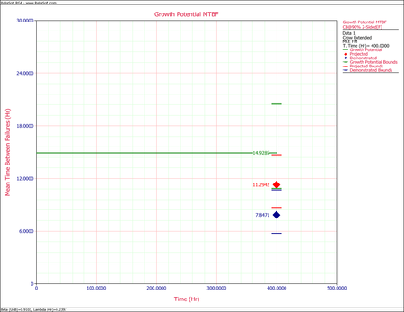
The figure below shows the Fisher Matrix confidence bounds at the 90% confidence level for the demonstrated, projected and growth potential MTBF.
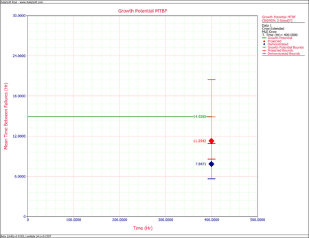
The next figure shows these bounds based on the Crow method.


