Crow Extended Model Examples
 |
New format available! This reference is now available in a new format that offers faster page load, improved display for calculations and images and more targeted search.
As of January 2024, this Reliawiki page will not continue to be updated. Please update all links and bookmarks to the latest references at RGA examples and RGA reference examples.
These examples appear in the Reliability Growth and Repairable System Analysis Reference book.
Parameter Estimation for Test-Find-Test Data
Consider the data in the first table below. A system was tested for [math]\displaystyle{ T=400\,\! }[/math] hours. There were a total of [math]\displaystyle{ N=42\,\! }[/math] failures and all corrective actions will be delayed until after the end of the 400 hour test. Each failure has been designated as either an A failure mode (the cause will not receive a corrective action) or a BD mode (the cause will receive a corrective action). There are [math]\displaystyle{ {{N}_{A}}=10\,\! }[/math] A mode failures and [math]\displaystyle{ {{N}_{BD}}=32\,\! }[/math] BD mode failures. In addition, there are [math]\displaystyle{ M=16\,\! }[/math] distinct BD failure modes, which means 16 distinct corrective actions will be incorporated into the system at the end of test. The total number of failures for the [math]\displaystyle{ {{j}^{th}}\,\! }[/math] observed distinct BD mode is denoted by [math]\displaystyle{ {{N}_{j}}\,\! }[/math], and the total number of BD failures during the test is [math]\displaystyle{ {{N}_{BD}}=\underset{j=1}{\overset{M}{\mathop{\sum }}}\,{{N}_{j}}\,\! }[/math]. These values and effectiveness factors are given in the second table
Do the following:
- Determine the projected MTBF and failure intensity.
- Determine the growth potential MTBF and failure intensity.
- Determine the demonstrated MTBF and failure intensity.
| Test-Find-Test Data | ||||||
| [math]\displaystyle{ i\,\! }[/math] | [math]\displaystyle{ {{X}_{i}}\,\! }[/math] | Mode | [math]\displaystyle{ i\,\! }[/math] | [math]\displaystyle{ {{X}_{i}}\,\! }[/math] | Mode | |
|---|---|---|---|---|---|---|
| 1 | 15 | BD1 | 22 | 260.1 | BD1 | |
| 2 | 25.3 | BD2 | 23 | 263.5 | BD8 | |
| 3 | 47.5 | BD3 | 24 | 273.1 | A | |
| 4 | 54 | BD4 | 25 | 274.7 | BD6 | |
| 5 | 56.4 | BD5 | 26 | 285 | BD13 | |
| 6 | 63.6 | A | 27 | 304 | BD9 | |
| 7 | 72.2 | BD5 | 28 | 315.4 | BD4 | |
| 8 | 99.6 | BD6 | 29 | 317.1 | A | |
| 9 | 100.3 | BD7 | 30 | 320.6 | A | |
| 10 | 102.5 | A | 31 | 324.5 | BD12 | |
| 11 | 112 | BD8 | 32 | 324.9 | BD10 | |
| 12 | 120.9 | BD2 | 33 | 342 | BD5 | |
| 13 | 125.5 | BD9 | 34 | 350.2 | BD3 | |
| 14 | 133.4 | BD10 | 35 | 364.6 | BD10 | |
| 15 | 164.7 | BD9 | 36 | 364.9 | A | |
| 16 | 177.4 | BD10 | 37 | 366.3 | BD2 | |
| 17 | 192.7 | BD11 | 38 | 373 | BD8 | |
| 18 | 213 | A | 39 | 379.4 | BD14 | |
| 19 | 244.8 | A | 40 | 389 | BD15 | |
| 20 | 249 | BD12 | 41 | 394.9 | A | |
| 21 | 250.8 | A | 42 | 395.2 | BD16 | |
| Effectiveness Factors for the Unique BD Modes | |||
| BD Mode | Number [math]\displaystyle{ {{N}_{j}}\,\! }[/math] | First Occurrence | EF [math]\displaystyle{ {{d}_{i}}\,\! }[/math] |
|---|---|---|---|
| 1 | 2 | 15.0 | .67 |
| 2 | 3 | 25.3 | .72 |
| 3 | 2 | 47.5 | .77 |
| 4 | 2 | 54.0 | .77 |
| 5 | 3 | 54.0 | .87 |
| 6 | 2 | 99.6 | .92 |
| 7 | 1 | 100.3 | .50 |
| 8 | 3 | 112.0 | .85 |
| 9 | 3 | 125.5 | .89 |
| 10 | 4 | 133.4 | .74 |
| 11 | 1 | 192.7 | .70 |
| 12 | 2 | 249.0 | .63 |
| 13 | 1 | 285.0 | .64 |
| 14 | 1 | 379.4 | .72 |
| 15 | 1 | 389.0 | .69 |
| 16 | 1 | 395.2 | .46 |
Solution
- The maximum likelihood estimates of [math]\displaystyle{ {{\beta }_{BD}}\,\! }[/math] and [math]\displaystyle{ {{\lambda }_{BD}}\,\! }[/math] are determined to be:
- [math]\displaystyle{ \begin{align} {{{\hat{\beta }}}_{BD}} = & \frac{M}{\underset{i=1}{\overset{M}{\mathop{\sum }}}\,\ln (\tfrac{T}{{{X}_{i}}})} \\ = & 0.7970 \\ {{{\hat{\lambda }}}_{BD}} = & 0.1350 \end{align}\,\! }[/math]
- [math]\displaystyle{ \begin{align} {{\overline{\beta }}_{BD}} = & \frac{M-1}{M}{{{\hat{\beta }}}_{BD}} \\ = & 0.7472 \end{align}\,\! }[/math]
- [math]\displaystyle{ \begin{align} r(T) = & \left( \frac{{{N}_{A}}}{T}+\underset{i=1}{\overset{M}{\mathop \sum }}\,(1-{{d}_{i}})\frac{{{N}_{i}}}{T} \right)+\overline{d}\left( \frac{M}{T}{{\overline{\beta }}_{BD}} \right) \\ = & 0.0661 \end{align}\,\! }[/math]
- [math]\displaystyle{ M\widehat{T}B{{F}_{P}}={{[r(T)]}^{-1}}=15.127\,\! }[/math]
- To estimate the maximum reliability that can be attained with this management strategy, use the following calculations.
- [math]\displaystyle{ \begin{align} {{N}_{A}}/T=0.0250 \end{align}\,\! }[/math]
- [math]\displaystyle{ \frac{1}{T}\underset{i=1}{\overset{16}{\mathop \sum }}\,(1-{{d}_{i}}){{N}_{i}}=0.0196\,\! }[/math]
- [math]\displaystyle{ \begin{align} {{\widehat{r}}_{GP}}(T) = & \left( \frac{{{N}_{A}}}{T}+\underset{i=1}{\overset{M}{\mathop \sum }}\,(1-{{d}_{i}})\frac{{{N}_{i}}}{T} \right) \\ = & 0.0250+0.0196 \\ = & 0.0446 \end{align}\,\! }[/math]
- [math]\displaystyle{ M\widehat{T}B{{F}_{GP}}={{[{{\widehat{r}}_{GP}}]}^{-1}}=22.4467\,\! }[/math]
- The demonstrated failure intensity and MTBF are estimated by:
- [math]\displaystyle{ \begin{align} {{\widehat{\lambda }}_{D}}(T) = & \frac{{{N}_{A}}+{{N}_{BD}}}{T} \\ = & \frac{42}{400} \\ = & 0.1050 \end{align}\,\! }[/math]
- [math]\displaystyle{ \begin{align} M\widehat{T}B{{F}_{D}} = & {{[{{\widehat{\lambda }}_{D}}(T)]}^{-1}} \\ = & 9.5238 \end{align}\,\! }[/math]


Confidence Bounds
Calculate the 2-sided 90% confidence bounds on the demonstrated, projected and growth potential failure intensity for the Test-Find-Test data given above.
Solution
The estimated demonstrated failure intensity is [math]\displaystyle{ {{\widehat{\lambda }}_{D}}(T)=\tfrac{{{N}_{A}}+{{N}_{B}}}{T}=0.1050\,\! }[/math]. Based on this value, the Fisher Matrix confidence bounds for the demonstrated failure intensity at the 90% confidence level are:
- [math]\displaystyle{ \begin{align} {{[{{\lambda }_{D}}(T)]}_{L}} = & {{{\hat{\lambda }}}_{D}}(T)+\frac{{{C}^{2}}}{2}-\sqrt{{{{\hat{\lambda }}}_{D}}(T){{C}^{2}}+\frac{{{C}^{4}}}{4}} \\ = & 0.08152 \end{align}\,\! }[/math]
- [math]\displaystyle{ \begin{align} {{[{{\lambda }_{D}}(T)]}_{U}} = & {{{\hat{\lambda }}}_{D}}(T)+\frac{{{C}^{2}}}{2}+\sqrt{{{{\hat{\lambda }}}_{D}}(T){{C}^{2}}+\frac{{{C}^{4}}}{4}} \\ = & 0.13525 \end{align}\,\! }[/math]
The Crow confidence bounds for the demonstrated failure intensity at the 90% confidence level are:
- [math]\displaystyle{ \begin{align} {{[{{\lambda }_{D}}(T)]}_{L}} = & {{\widehat{\lambda }}_{D}}(T)\frac{\chi _{(2N,1-\alpha /2)}^{2}}{2N} \\ = & 0.07985 \\ {{[{{\lambda }_{D}}(T)]}_{U}} = & {{\widehat{\lambda }}_{D}}(T)\frac{\chi _{(2N,\alpha /2)}^{2}}{2N} \\ = & 0.13299 \end{align}\,\! }[/math]
The projected failure intensity is:
- [math]\displaystyle{ \begin{align} \hat{\lambda_{p}} &= \frac{N_{i}}{T}+\sum_{i=1}^{M}(1-d_{i})\frac{N}{T}+\overline{d}\left(\frac{M}{T}\overline{\beta} \right )\\ &= 0.06611 \end{align} }[/math]
Based on this value, the Fisher Matrix confidence bounds at the 90% confidence level for the projected failure intensity are:
- [math]\displaystyle{ \begin{align} {{[{{{\hat{\lambda }}}_{P}}(T)]}_{L}} = & {{{\hat{\lambda }}}_{P}}(T){{e}^{{{z}_{\alpha }}\sqrt{Var({{{\hat{\lambda }}}_{P}}(T))}/{{{\hat{\lambda }}}_{P}}(T)}} \\ = & 0.04902 \end{align}\,\! }[/math]
- [math]\displaystyle{ \begin{align} {{[{{{\hat{\lambda }}}_{P}}(T)]}_{U}} = & {{{\hat{\lambda }}}_{P}}(T){{e}^{-{{z}_{\alpha }}\sqrt{Var({{{\hat{\lambda }}}_{P}}(T))}/{{{\hat{\lambda }}}_{P}}(T)}} \\ = & 0.08915 \end{align}\,\! }[/math]
The Crow confidence bounds for the projected failure intensity are:
- [math]\displaystyle{ \begin{align} {{[{{\lambda }_{P}}(T)]}_{L}} = & {{{\hat{\lambda }}}_{P}}(T)+\frac{{{C}^{2}}}{2}-\sqrt{{{{\hat{\lambda }}}_{P}}(T)\cdot {{C}^{2}}+\frac{{{C}^{4}}}{4}} \\ = & 0.04807 \\ {{[{{\lambda }_{P}}(T)]}_{U}} = & {{{\hat{\lambda }}}_{P}}(T)+\frac{{{C}^{2}}}{2}+\sqrt{{{{\hat{\lambda }}}_{P}}(T)\cdot \ \,{{C}^{2}}+\frac{{{C}^{4}}}{4}} \\ = & 0.09090 \end{align}\,\! }[/math]
The growth potential failure intensity is:
- [math]\displaystyle{ \widehat{r}_{GP} (T) = \left (\frac{N_A}{T} + \sum_{i=1}^M (1-d_i) \tfrac{N_i}{T} \right ) = 0.04455 \,\! }[/math].
Based on this value, the Fisher Matrix and Crow confidence bounds at the 90% confidence level for the growth potential failure intensity are:
- [math]\displaystyle{ \begin{align} {{r}_{L}} = & {{{\hat{r}}}_{GP}}+\frac{{{C}^{2}}}{2}-\sqrt{{{{\hat{r}}}_{GP}}{{C}^{2}}+\frac{{{C}^{4}}}{4}} \\ = & 0.03020 \\ {{r}_{U}} = & {{{\hat{r}}}_{GP}}+\frac{{{C}^{2}}}{2}+\sqrt{{{{\hat{r}}}_{GP}}{{C}^{2}}+\frac{{{C}^{4}}}{4}} \\ = & 0.0656 \end{align}\,\! }[/math]
The figure below shows the Fisher Matrix confidence bounds at the 90% confidence level for the demonstrated, projected and growth potential failure intensity.

The following figure shows these bounds based on the Crow method.

Parameter Estimation for Test-Fix-Find-Test Data
Consider the data given in the first table below. There were 56 total failures and [math]\displaystyle{ T=400\,\! }[/math]. The effectiveness factors of the unique BD modes are given in the second table. Determine the following:
- Calculate the demonstrated MTBF and failure intensity.
- Calculate the projected MTBF and failure intensity.
- What is the rate at which unique BD modes are being generated during this test?
- If the test continues for an additional 50 hours, what is the minimum number of new unique BD modes expected to be generated?
| Test-Fix-Find-Test Data | |||||
| [math]\displaystyle{ i\,\! }[/math] | [math]\displaystyle{ {{X}_{i}}\,\! }[/math] | Mode | [math]\displaystyle{ i\,\! }[/math] | [math]\displaystyle{ {{X}_{i}}\,\! }[/math] | Mode |
|---|---|---|---|---|---|
| 1 | 0.7 | BC17 | 29 | 192.7 | BD11 |
| 2 | 3.7 | BC17 | 30 | 213 | A |
| 3 | 13.2 | BC17 | 31 | 244.8 | A |
| 4 | 15 | BD1 | 32 | 249 | BD12 |
| 5 | 17.6 | BC18 | 33 | 250.8 | A |
| 6 | 25.3 | BD2 | 34 | 260.1 | BD1 |
| 7 | 47.5 | BD3 | 35 | 263.5 | BD8 |
| 8 | 54 | BD4 | 36 | 273.1 | A |
| 9 | 54.5 | BC19 | 37 | 274.7 | BD6 |
| 10 | 56.4 | BD5 | 38 | 282.8 | BC27 |
| 11 | 63.6 | A | 39 | 285 | BD13 |
| 12 | 72.2 | BD5 | 40 | 304 | BD9 |
| 13 | 99.2 | BC20 | 41 | 315.4 | BD4 |
| 14 | 99.6 | BD6 | 42 | 317.1 | A |
| 15 | 100.3 | BD7 | 43 | 320.6 | A |
| 16 | 102.5 | A | 44 | 324.5 | BD12 |
| 17 | 112 | BD8 | 45 | 324.9 | BD10 |
| 18 | 112.2 | BC21 | 46 | 342 | BD5 |
| 19 | 120.9 | BD2 | 47 | 350.2 | BD3 |
| 20 | 121.9 | BC22 | 48 | 355.2 | BC28 |
| 21 | 125.5 | BD9 | 49 | 364.6 | BD10 |
| 22 | 133.4 | BD10 | 50 | 364.9 | A |
| 23 | 151 | BC23 | 51 | 366.3 | BD2 |
| 24 | 163 | BC24 | 52 | 373 | BD8 |
| 25 | 164.7 | BD9 | 53 | 379.4 | BD14 |
| 26 | 174.5 | BC25 | 54 | 389 | BD15 |
| 27 | 177.4 | BD10 | 55 | 394.9 | A |
| 28 | 191.6 | BC26 | 56 | 395.2 | BD16 |
| Effectiveness Factors for the Unique BD Modes | |
| BD Mode | EF [math]\displaystyle{ {{d}_{i}}\,\! }[/math] |
|---|---|
| 1 | .67 |
| 2 | .72 |
| 3 | .77 |
| 4 | .77 |
| 5 | .87 |
| 6 | .92 |
| 7 | .50 |
| 8 | .85 |
| 9 | .89 |
| 10 | .74 |
| 11 | .70 |
| 12 | .63 |
| 13 | .64 |
| 14 | .72 |
| 15 | .69 |
| 16 | .46 |
Solution
- In order to obtain [math]\displaystyle{ {{\widehat{\lambda }}_{CA}}\,\! }[/math], use the traditional Crow-AMSAA model for test-fix-test to fit all 56 data points, regardless of the failure mode classification to get:
- [math]\displaystyle{ \begin{align} \widehat{\beta }= & 0.91026 \\ \widehat{\lambda }= & 0.23969 \end{align}\,\! }[/math]
- [math]\displaystyle{ \begin{align} {{\widehat{\lambda }}_{CA}} = & \widehat{\lambda }\widehat{\beta }{{T}^{\widehat{\beta }-1}} \\ = & 0.23969\times 0.91026\times {{400}^{(0.91026-1)}} \\ = & 0.12744 \end{align}\,\! }[/math]
- [math]\displaystyle{ {{\widehat{M}}_{CA}}={{[{{\widehat{\lambda }}_{CA}}]}^{-1}}=7.84708\,\! }[/math]
- For this data set, [math]\displaystyle{ M=16\,\! }[/math] and [math]\displaystyle{ T=400\,\! }[/math].
- [math]\displaystyle{ {{\widehat{\lambda }}_{BD}}=\frac{{{N}_{BD}}}{T}=\frac{32}{400}=0.08\,\! }[/math]
- [math]\displaystyle{ \overline{d}=\underset{i=1}{\overset{M}{\mathop \sum }}\,{{d}_{i}}/M=0.72125\,\! }[/math]
- [math]\displaystyle{ \underset{i=1}{\overset{16}{\mathop \sum }}\,(1-{{d}_{i}}){{N}_{i}}/T=0.01955\,\! }[/math]
- [math]\displaystyle{ \begin{align} {{{\hat{\beta }}}_{BD}}= & 0.74715 \\ {{{\hat{\lambda }}}_{BD}} = & 0.18197 \end{align}\,\! }[/math]
- [math]\displaystyle{ \overline{d}\widehat{h}(T|BD)=0.0215\,\! }[/math]
- [math]\displaystyle{ \begin{align} {{\widehat{\lambda }}_{EM}} = & {{\widehat{\lambda }}_{CA}}-{{\widehat{\lambda }}_{BD}}+\underset{i=1}{\overset{K}{\mathop \sum }}\,(1-{{d}_{i}})\frac{{{N}_{i}}}{T}+\overline{d}\widehat{h}(T|BD) \\ = & 0.12744-0.08+0.0196+0.0215 \\ = & 0.08854 \end{align}\,\! }[/math]
- [math]\displaystyle{ \begin{align} {{\widehat{M}}_{EM}} = & {{[{{\widehat{\lambda }}_{EM}}]}^{-1}} \\ = & 11.29418 \end{align}\,\! }[/math]
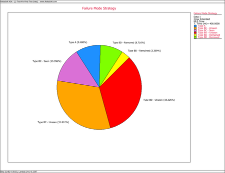
This pie chart shows that 9.48% of the system's failure intensity has been left in (A modes), 31.81% of the failure intensity due to the BC modes has not been seen yet and 13.40% was removed during the test (BC modes - seen). In addition, 33.23% of the failure intensity due to the BD modes has not been seen yet, 3.37% will remain in the system since the corrective actions will not be completely effective at eliminating the identified failure modes, and 8.72% will be removed after the delayed corrective actions.
- The rate at which unique BD modes are being generated is equal to [math]\displaystyle{ h{{(T|BD)}^{-1}}\,\! }[/math], where:
- [math]\displaystyle{ \begin{align} h{{(T|BD)}^{-1}} = & \frac{1}{{{\widehat{\lambda }}_{BD}}{{\widehat{\beta }}_{BD}}{{T}^{{{\widehat{\beta }}_{BD}}-1}}} \\ = & \frac{T}{M{{\widehat{\beta }}_{BD}}} \\ = & 33.4605 \end{align}\,\! }[/math]
- Unique BD modes are being generated every 33.4605 hours. If the test continues for another 50 hours, then at least one new unique BD mode would be expected to be seen from this additional testing.
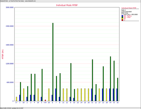
As shown in the next figure, the MTBF of each individual failure mode can be plotted, and the failure modes with the lowest MTBF can be identified. These are the failure modes that cause the majority of the system failures.


Confidence Bounds
Calculate the 2-sided confidence bounds at the 90% confidence level on the demonstrated, projected and growth potential MTBF for the Test-Fix-Find-Test data given above.
Solution
For this example, there are A, BC and BD failure modes, so the estimated demonstrated failure intensity, [math]\displaystyle{ {{\hat{\lambda }}_{D}}(T)\,\! }[/math], is simply the Crow-AMSAA model applied to all A, BC, and BD data.
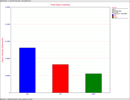
- [math]\displaystyle{ {{\hat{\lambda }}_{D}}(T)={{\widehat{\lambda }}_{CA}}=\widehat{\lambda }\widehat{\beta }{{T}^{\widehat{\beta }-1}}=0.12744\,\! }[/math]
Therefore, the demonstrated MTBF is:
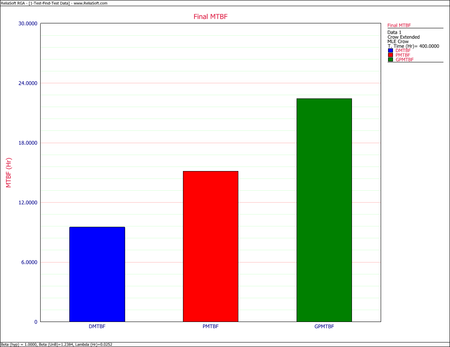
- [math]\displaystyle{ MTB{{F}_{D}}={{[{{\hat{\lambda }}_{D}}(T)]}^{-1}}=7.84708\,\! }[/math]
Based on this value, the Fisher Matrix confidence bounds for the demonstrated failure intensity at the 90% confidence level are:
- [math]\displaystyle{ \begin{align} {{[{{\lambda }_{D}}(T)]}_{L}} = & {{{\hat{\lambda }}}_{CA}}(T){{e}^{{{z}_{\alpha }}\sqrt{Var({{{\hat{\lambda }}}_{CA}}(T))}/{{{\hat{\lambda }}}_{CA}}(T)}} \\ = & 0.09339 \end{align}\,\! }[/math]
- [math]\displaystyle{ \begin{align} {{[{{\lambda }_{D}}(T)]}_{U}} = & {{{\hat{\lambda }}}_{CA}}(T){{e}^{-{{z}_{\alpha }}\sqrt{Var({{{\hat{\lambda }}}_{CA}}(T))}/{{{\hat{\lambda }}}_{CA}}(T)}} \\ = & 0.17390 \end{align}\,\! }[/math]
The Fisher Matrix confidence bounds for the demonstrated MTBF at the 90% confidence level are:
- [math]\displaystyle{ \begin{align} MTB{{F}_{{{D}_{L}}}} = & \frac{1}{{{[{{\lambda }_{D}}(T)]}_{U}}} \\ = & 5.75054 \\ MTB{{F}_{{{D}_{U}}}} = & \frac{1}{{{[{{\lambda }_{D}}(T)]}_{L}}} \\ = & 10.70799 \end{align}\,\! }[/math]
The Crow confidence bounds for the demonstrated MTBF at the 90% confidence level are:
- [math]\displaystyle{ \begin{align} MTB{{F}_{{{D}_{L}}}} = & \frac{1}{{{[{{\lambda }_{D}}(T)]}_{U}}} \\ = & \frac{1}{{{\widehat{\lambda }}_{D}}(T)\tfrac{{{\chi }^{2}}(2N,\alpha /2)}{2N}} \\ = & 5.6325 \\ MTB{{F}_{{{D}_{U}}}} = & \frac{1}{{{[{{\lambda }_{D}}(T)]}_{L}}} \\ = & \frac{1}{{{\widehat{\lambda }}_{D}}(T)\tfrac{{{\chi }^{2}}(2N,1-\alpha /2)}{2N}} \\ = & 10.8779 \end{align}\,\! }[/math]
The projected failure intensity is:
- [math]\displaystyle{ \begin{align} \hat{\lambda}_P (T) &= \widehat{\lambda}_{CA} - \widehat{\lambda}_{BD} + \sum_{i=1}^M (1-d_i) \tfrac{N_i}{T} + \bar{d}\widehat{h}(T|BD) \\ &= 0.0885 \,\! \end{align} }[/math]
Based on this value, the Fisher Matrix confidence bounds at the 90% confidence level for the projected failure intensity are:
- [math]\displaystyle{ \begin{align} {{[{{\lambda }_{P}}(T)]}_{L}} = & {{{\hat{\lambda }}}_{P}}(T){{e}^{{{z}_{\alpha }}\sqrt{Var({{{\hat{\lambda }}}_{P}}(T))}/{{{\hat{\lambda }}}_{P}}(T)}} \\ = & 0.0681 \end{align}\,\! }[/math]
- [math]\displaystyle{ \begin{align} {{[{{\lambda }_{P}}(T)]}_{U}} = & {{{\hat{\lambda }}}_{P}}(T){{e}^{-{{z}_{\alpha }}\sqrt{Var({{{\hat{\lambda }}}_{P}}(T))}/{{{\hat{\lambda }}}_{P}}(T)}} \\ = & 0.1152 \end{align}\,\! }[/math]
The Fisher Matrix confidence bounds for the projected MTBF at the 90% confidence level are:
- [math]\displaystyle{ \begin{align} MTB{{F}_{{{P}_{L}}}} = & \frac{1}{{{[{{\lambda }_{P}}(T)]}_{U}}} \\ = & 8.6818 \\ MTB{{F}_{{{P}_{U}}}} = & \frac{1}{{{[{{\lambda }_{P}}(T)]}_{L}}} \\ = & 14.6926 \end{align}\,\! }[/math]
The Crow confidence bounds for the projected failure intensity are:
- [math]\displaystyle{ \begin{align} {{[{{\lambda }_{P}}(T)]}_{L}} = & {{{\hat{\lambda }}}_{P}}(T)+\frac{{{C}^{2}}}{2}-\sqrt{{{{\hat{\lambda }}}_{P}}(T)\cdot \ \,{{C}^{2}}+\frac{{{C}^{4}}}{4}} \\ = & 0.0672 \\ {{[{{\lambda }_{P}}(T)]}_{U}} = & {{{\hat{\lambda }}}_{P}}(T)+\frac{{{C}^{2}}}{2}+\sqrt{{{{\hat{\lambda }}}_{P}}(T)\cdot {{C}^{2}}+\frac{{{C}^{4}}}{4}} \\ = & 0.1166 \end{align}\,\! }[/math]
The Crow confidence bounds for the projected MTBF at the 90% confidence level are:
- [math]\displaystyle{ \begin{align} MTB{{F}_{{{P}_{L}}}} = & \frac{1}{{{[{{\widehat{\lambda }}_{P}}(T)]}_{U}}} \\ = & 8.5743 \\ MTB{{F}_{{{P}_{U}}}} = & \frac{1}{{{[{{\widehat{\lambda }}_{P}}(T)]}_{L}}} \\ = & 14.8769 \end{align}\,\! }[/math]
The growth potential failure intensity is:
- [math]\displaystyle{ \widehat{\lambda}_{GP} = \widehat{\lambda}_{CA} - \widehat{\lambda}_{BD} + \sum_{i=1}^M (1-d_i) \tfrac{N_i}{T} = 0.0670 \,\! }[/math]
Based on this value, the Fisher Matrix and Crow confidence bounds at the 90% confidence level for the growth potential failure intensity are:
- [math]\displaystyle{ \begin{align} {{r}_{L}} = & {{{\hat{r}}}_{GP}}+\frac{{{C}^{2}}}{2}-\sqrt{{{{\hat{r}}}_{GP}}{{C}^{2}}+\frac{{{C}^{4}}}{4}} \\ = & 0.0488 \\ {{r}_{U}} = & {{{\hat{r}}}_{GP}}+\frac{{{C}^{2}}}{2}+\sqrt{{{{\hat{r}}}_{GP}}{{C}^{2}}+\frac{{{C}^{4}}}{4}} \\ = & 0.0919 \end{align}\,\! }[/math]
The Fisher Matrix and Crow confidence bounds for the growth potential MTBF at the 90% confidence level are:
- [math]\displaystyle{ \begin{align} MTB{{F}_{G{{P}_{L}}}} = & \frac{1}{{{r}_{U}}} \\ = & 10.8790 \\ MTB{{F}_{G{{P}_{U}}}} = & \frac{1}{{{r}_{L}}} \\ = & 20.4855 \end{align}\,\! }[/math]
The figure below shows the Fisher Matrix confidence bounds at the 90% confidence level for the demonstrated, projected and growth potential MTBF.

The next figure shows these bounds based on the Crow method.
