Duane Confidence Bounds Example: Difference between revisions
No edit summary |
No edit summary |
||
| Line 106: | Line 106: | ||
:<math>\begin{align} | :<math>\begin{align} | ||
{{m}_{c}}{{(t)}_{l}}= & | {{m}_{c}}{{(t)}_{l}}= & 855.9815 \\ | ||
{{m}_{c}}{{(t)}_{u}}= & | {{m}_{c}}{{(t)}_{u}}= & 936.5071 | ||
\end{align}\,\!</math> | \end{align}\,\!</math> | ||
| Line 113: | Line 113: | ||
:<math>\begin{align} | :<math>\begin{align} | ||
{{m}_{i}}{{(t)}_{l}}= & | {{m}_{i}}{{(t)}_{l}}= & 2213.1753 \\ | ||
{{m}_{i}}{{(t)}_{u}}= & | {{m}_{i}}{{(t)}_{u}}= & 2421.3776 | ||
\end{align}\,\!</math> | \end{align}\,\!</math> | ||
Revision as of 19:55, 8 August 2018
 |
New format available! This reference is now available in a new format that offers faster page load, improved display for calculations and images and more targeted search.
As of January 2024, this Reliawiki page will not continue to be updated. Please update all links and bookmarks to the latest references at RGA examples and RGA reference examples.
This example appears in the Reliability Growth and Repairable System Analysis Reference.
Using the values of [math]\displaystyle{ \hat{b}\,\! }[/math] and [math]\displaystyle{ \hat{\alpha }\,\! }[/math] estimated from the least squares analysis in Least Squares Example 2:
- [math]\displaystyle{ \hat{b}=1.9453\,\! }[/math]
- [math]\displaystyle{ \hat{\alpha}=0.6133\,\! }[/math]
Calculate the 90% confidence bounds for the following:
- The parameters [math]\displaystyle{ \alpha\,\! }[/math] and [math]\displaystyle{ b\,\! }[/math].
- The cumulative and instantaneous failure intensity.
- The cumulative and instantaneous MTBF.
Solution
- Use the values of [math]\displaystyle{ \hat{b}\,\! }[/math] and [math]\displaystyle{ \hat{\alpha }\,\! }[/math] estimated from the least squares analysis. Then:
- [math]\displaystyle{ \begin{align} {{S}_{xx}}&=\left[ \underset{i=1}{\overset{n}{\mathop \sum }}\,{{(\ln {{t}_{i}})}^{2}} \right]-\frac{1}{n}{{\left( \underset{i=1}{\overset{n}{\mathop \sum }}\,\ln ({{t}_{i}}) \right)}^{2}} \\ & = 1400.9084-1301.4545 \\ & = 99.4539 \end{align}\,\! }[/math]
- [math]\displaystyle{ \begin{align} SE(\hat{\alpha })= & \frac{\sigma }{\sqrt{{{S}_{xx}}}} \\ = & \frac{0.08428}{9.9727} \\ = & 0.008452 \end{align}\,\! }[/math]
- [math]\displaystyle{ \begin{align} SE(\ln \hat{b})= & \sigma \cdot \sqrt{\frac{\underset{i=1}{\overset{n}{\mathop{\sum }}}\,{{(\ln {{T}_{i}})}^{2}}}{n\cdot {{S}_{xx}}}} \\ = & 0.065960 \end{align}\,\! }[/math]
- [math]\displaystyle{ C{{B}_{\alpha }}=\hat{\alpha }\pm {{t}_{n-2,\alpha /2}}SE(\hat{\alpha })\,\! }[/math]
- [math]\displaystyle{ \begin{align} {{\alpha }_{L}}= & 0.602050 \\ {{\alpha }_{U}}= & 0.624417 \end{align}\,\! }[/math]
- [math]\displaystyle{ C{{B}_{b}}=\hat{b}{{e}^{\pm {{t}_{n-2,\alpha /2}}SE\left[ \ln (\hat{b}) \right]}}\,\! }[/math]
- [math]\displaystyle{ \begin{align} {{b}_{L}}= & 1.7831 \\ {{b}_{U}}= & 2.1231 \end{align}\,\! }[/math]
- The cumulative failure intensity is:
- [math]\displaystyle{ \begin{align} {{\lambda }_{c}}= & \frac{1}{1.9453}\cdot {{22000}^{-0.6133}} \\ = & 0.00111689 \end{align}\,\! }[/math]
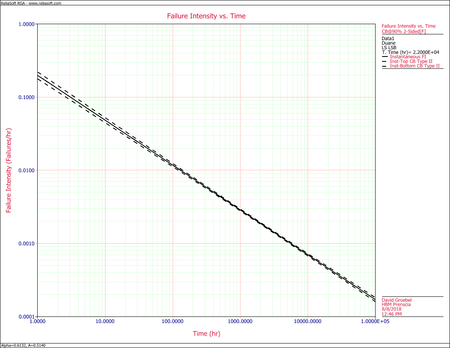
- [math]\displaystyle{ \begin{align} {{\lambda }_{i}}= & \frac{1}{1.9453}\cdot (1-0.6133)\cdot {{22000}^{-0.6133}} \\ = & 0.00043198 \end{align}\,\! }[/math]
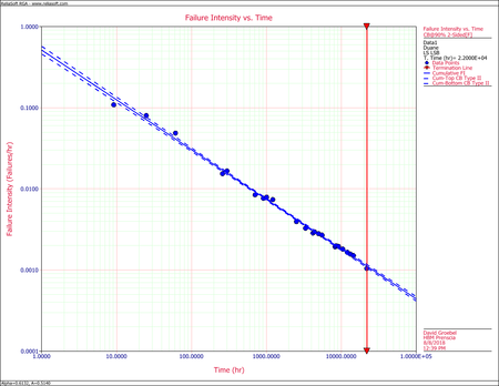
- [math]\displaystyle{ \begin{align} {{[{{\lambda }_{c}}(t)]}_{L}}= & 0.00106780 \\ {{[{{\lambda }_{c}}(t)]}_{U}}= & 0.00116825 \end{align}\,\! }[/math]
- [math]\displaystyle{ \begin{align} {{[{{\lambda }_{i}}(t)]}_{L}}= & 0.00041299 \\ {{[{{\lambda }_{c}}(t)]}_{U}}= & 0.00045184 \end{align}\,\! }[/math]
- The cumulative MTBF is:
- [math]\displaystyle{ \begin{align} {{m}_{c}}(T)= & 1.9453\cdot {{22000}^{0.6133}} \\ = & 895.3395 \end{align}\,\! }[/math]
- [math]\displaystyle{ \begin{align} {{m}_{i}}(T)= & \frac{1.9453}{1-0.6133}\cdot {{22000}^{0.6133}} \\ = & 2314.9369 \end{align}\,\! }[/math]
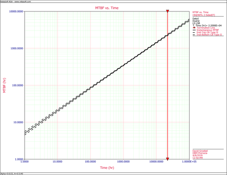
- [math]\displaystyle{ \begin{align} {{m}_{c}}{{(t)}_{l}}= & 855.9815 \\ {{m}_{c}}{{(t)}_{u}}= & 936.5071 \end{align}\,\! }[/math]
- [math]\displaystyle{ \begin{align} {{m}_{i}}{{(t)}_{l}}= & 2213.1753 \\ {{m}_{i}}{{(t)}_{u}}= & 2421.3776 \end{align}\,\! }[/math]
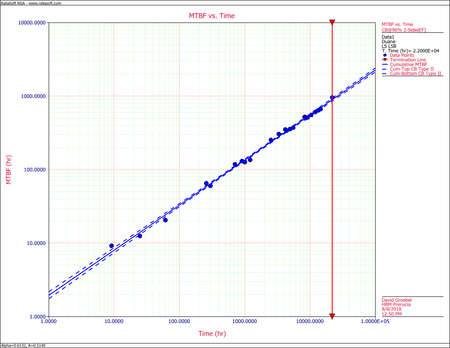
The next figure displays the instantaneous MTBF. Both are plotted with confidence bounds.