Example: CFM-Weibull

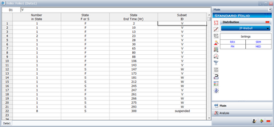
From Meeker & Escobar [27], the following table gives failure times for an electric component that has two failure modes.

One failure mode is due to random voltage spikes which cause failure by overloading the system (denoted as a [math]\displaystyle{ V }[/math] in the table). The other failure mode is due to wear-out failures which usually happen only after the system has run for many cycles (this failure mode is denoted as a [math]\displaystyle{ W }[/math] in the table).

Considering that these are competing failure modes, determine the overall reliability for the component at 100,000 cycles.

[math]\displaystyle{ \begin{matrix} Number & Failure & Failure & Number & Failure & Failure \\ in State & Time* & Mode & in State & Time* & Mode \\ \text{1} & \text{2} & \text{V} & \text{1} & \text{147} & \text{W} \\ \text{1} & \text{10} & \text{V} & \text{1} & \text{173} & \text{V} \\ \text{1} & \text{13} & \text{V} & \text{1} & \text{181} & \text{W} \\ \text{2} & \text{23} & \text{V} & \text{1} & \text{212} & \text{W} \\ \text{1} & \text{28} & \text{V} & \text{1} & \text{245} & \text{W} \\ \text{1} & \text{30} & \text{V} & \text{1} & \text{247} & \text{V} \\ \text{1} & \text{65} & \text{V} & \text{1} & \text{261} & \text{V} \\ \text{1} & \text{80} & \text{V} & \text{1} & \text{266} & \text{W} \\ \text{1} & \text{88} & \text{V} & \text{1} & \text{275} & \text{W} \\ \text{1} & \text{106} & \text{V} & \text{1} & \text{293} & \text{W} \\ \text{1} & \text{143} & \text{V} & \text{8} & \text{300} & \text{suspended} \\ \end{matrix} }[/math]

• Failure times given are in thousands of cycles.

Solution

We will begin by performing a Weibull analysis of the voltage spike ( [math]\displaystyle{ V }[/math] ) failure mode. In order to do this, we must consider all of the failures for the wear-out mode to be suspensions. The input data for the analysis are shown next:

Analyzing this data set using the maximum likelihood method (recommended due to the number of suspensions in the data) and assuming a Weibull distribution, we obtain the parameters [math]\displaystyle{ {{\beta }_{V}}=0.6711 }[/math] and [math]\displaystyle{ {{\eta }_{V}}=449.4 }[/math] . The reliability for this failure mode at [math]\displaystyle{ t=100 }[/math] is [math]\displaystyle{ {{R}_{V}}(100)=0.694 }[/math] .

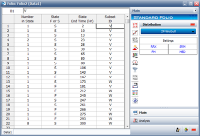
We follow an identical procedure for the wear-out failure mode, counting only the [math]\displaystyle{ W }[/math] entries as failures and assuming the [math]\displaystyle{ V }[/math] entries are suspensions. This is shown next.

Once again, analyzing with a Weibull distribution with maximum likelihood estimators, we obtain the parameters [math]\displaystyle{ {{\beta }_{W}}=4.337 }[/math] and [math]\displaystyle{ {{\eta }_{W}}=340.4 }[/math] . The reliability for this failure mode at [math]\displaystyle{ t=100 }[/math] is [math]\displaystyle{ {{R}_{W}}(100)=0.995 }[/math] .

We can now use Eqn. (sysrel) to determine the overall system reliability at 100,000 cycles:

[math]\displaystyle{ \begin{align} & {{R}_{sys}}(100)= & {{R}_{V}}(100)\cdot {{R}_{W}}(100) \\ & = & 0.694\cdot 0.995 \\ & = & 0.69053 \end{align} }[/math]

Or the reliability of the unit (or system) under both modes is [math]\displaystyle{ {{R}_{sys}}(100)=69.053%. }[/math]

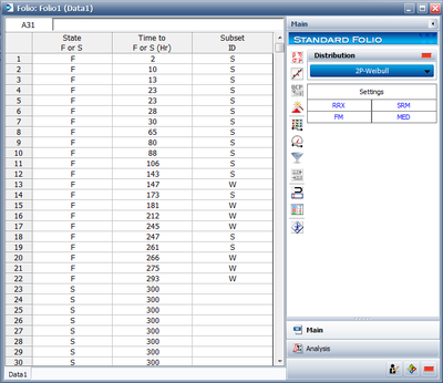
Note that Weibull++ can perform this analysis for you automatically. To accomplish this, the data would be entered in a single data sheet and competing failure modes chosen as the analysis method. This is shown in the next graphic.

CFM Weibull Example

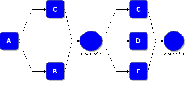
Assume that a product has five failure modes: A, B, C, D and F. Furthermore, assume that failure of the product will occur if mode A occurs, modes B and C occur simultaneously or if either modes C and D, C and F or D and F occur simultaneously. Times-to-failure for each mode is given in the next table.

[math]\displaystyle{ \begin{matrix} \text{TTF for A} & \text{TTF for B} & \text{TTF for C} & \text{TTF for D} & \text{TTF for F} \\ \text{276} & \text{23} & \text{499} & \text{467} & \text{67} \\ \text{320} & \text{36} & \text{545} & \text{540} & \text{72} \\ \text{323} & \text{57} & \text{661} & \text{716} & \text{81} \\ \text{558} & \text{89} & \text{738} & \text{737} & \text{108} \\ \text{674} & \text{99} & \text{987} & \text{761} & \text{110} \\ \text{829} & \text{154} & \text{1165} & \text{1093} & \text{127} \\ \text{878} & \text{200} & \text{1337} & \text{1283} & \text{148} \\ \end{matrix} }[/math]

The RBD that describes this configuration is shown next.

[math]\displaystyle{ }[/math]

One folio with multiple data sheets was created in Weibull++ for each of the data sets and each file was analyzed using the two-parameter Weibull distribution, MLE as the analysis method and Fisher Matrix as the confidence bounds method. A diagram is created by choosing Add Diagram from the Project menu. The failure modes can be inserted into the diagram by dragging them from the template. The nodes are inserted by clicking choosing Add Node from the Diagram menu.

[math]\displaystyle{ }[/math]

The number of required paths can be specified by double clicking the node and entering the appropriate number (1 in the first node and 2 in the second node).

[math]\displaystyle{ }[/math]

Using the Quick Calculation Pad (QCP), the estimated R( [math]\displaystyle{ 100 }[/math] hours [math]\displaystyle{ ) }[/math] and the 90% two-sided confidence bounds are:

[math]\displaystyle{ \begin{matrix} {{{\hat{R}}}_{U}}(100)=0.991 \\ \hat{R}(100)=0.9905 \\ {{{\hat{R}}}_{L}}(100)=0.9080 \\ \end{matrix} }[/math]