Exponential Distribution for Grouped Data Example

New format available! This reference is now available in a new format that offers faster page load, improved display for calculations and images and more targeted search.

As of January 2024, this Reliawiki page will not continue to be updated. Please update all links and bookmarks to the latest references at Weibull examples and Weibull reference examples.

---

This example appears in the Life Data Analysis Reference book.

Twenty units were reliability tested with the following results:

Table - Life Test Data
Number of Units in Group	Time-to-Failure
7	100
5	200
3	300
2	400
1	500
2	600

1. Assuming a 2-parameter exponential distribution, estimate the parameters by hand using the MLE analysis method.

2. Repeat the above using Weibull++. (Enter the data as grouped data to duplicate the results.)

3. Show the Probability plot for the analysis results.

4. Show the Reliability vs. Time plot for the results.

5. Show the pdf plot for the results.

6. Show the Failure Rate vs. Time plot for the results.

7. Estimate the parameters using the rank regression on Y (RRY) analysis method (and using grouped ranks).

Solution

1. For the 2-parameter exponential distribution and for [math]\displaystyle{ \hat{\gamma }=100 }[/math] hours (first failure), the partial of the log-likelihood function, [math]\displaystyle{ \lambda }[/math], becomes:

[math]\displaystyle{ \begin{align} \frac{\partial \Lambda }{\partial \lambda }= &\underset{i=1}{\overset{6}{\mathop \sum }}\,{N_i} \left[ \frac{1}{\lambda }-\left( {{T}_{i}}-100 \right) \right]=0\\ \Rightarrow & 7[\frac{1}{\lambda }-(100-100)]+5[\frac{1}{\lambda}-(200-100)] + \ldots +2[\frac{1}{\lambda}-(600-100)]\\ = & 0\\ \Rightarrow & \hat{\lambda}=\frac{20}{3100}=0.0065 \text{fr/hr} \end{align} }[/math]

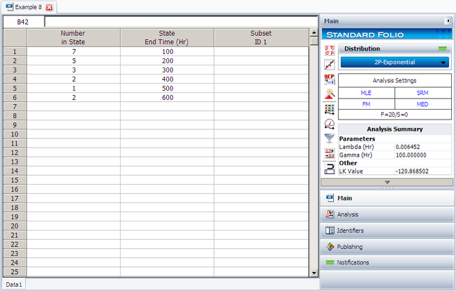
2. Enter the data in a Weibull++ standard folio and calculate it as shown next.

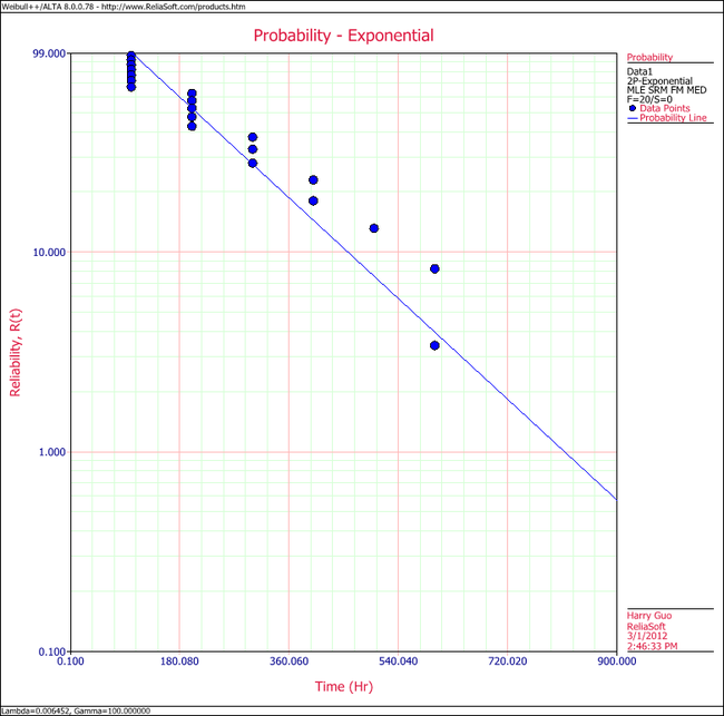
3. The exponential probability plot is shown next

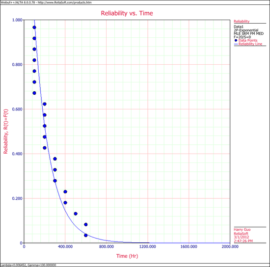
The Plot Type drop-down box allows you to select different plot types, shown next.

4. Select Reliability vs. Time.

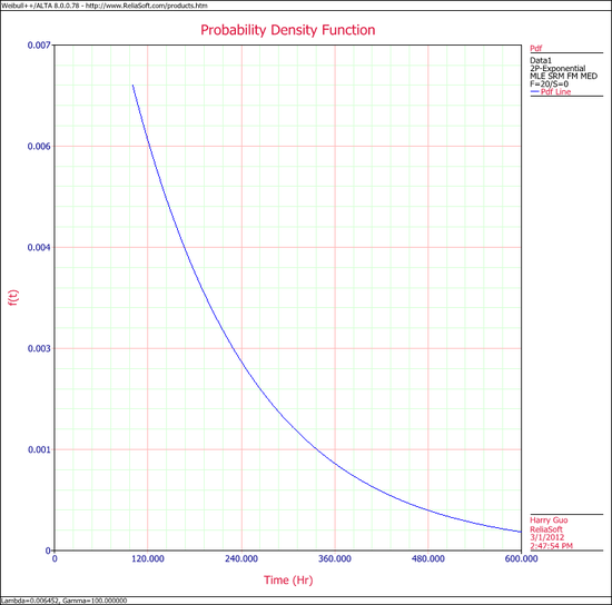
5. The exponential [math]\displaystyle{ pdf }[/math] plot is shown next.

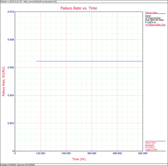
6. The exponential failure rate plot is shown next.

Note that, as described at the beginning of this chapter, the failure rate for the exponential distribution is constant. Also note that the failure rate plot does not exist for times before the location parameter, [math]\displaystyle{ \gamma }[/math], at 100 hours.

7. In the case of grouped data, one must be cautious when estimating the parameters using a rank regression method. That is because the median rank values are determined from the total number of failures observed by time [math]\displaystyle{ {{T}_{i}} }[/math] where [math]\displaystyle{ i }[/math] indicates the group number. In this example the total number of groups is [math]\displaystyle{ N=6 }[/math] and the total number of units is [math]\displaystyle{ {{N}_{T}}=20 }[/math]. Thus, the median rank values will be estimated for twenty units and for the total failed units ([math]\displaystyle{ {{N}_{{{F}_{i}}}} }[/math]) up to the [math]\displaystyle{ {{i}^{th}} }[/math] group, for the [math]\displaystyle{ {{i}^{th}} }[/math] rank value. The median ranks values can be found from rank tables or they can be estimated using ReliaSoft's Quick Statistical Reference.

For example, the median rank value of the fourth group will be the [math]\displaystyle{ {{17}^{th}} }[/math] rank out of a sample size of twenty units (or 81.945%).

The following table is then constructed.

[math]\displaystyle{ \begin{matrix} N & {{N}_{F}} & {{N}_{{{F}_{i}}}} & {{T}_{i}} & F({{T}_{i}}) & {{y}_{i}} & T_{i}^{2} & y_{i}^{2} & {{T}_{i}}{{y}_{i}} \\ \text{1} & \text{7} & \text{7} & \text{100} & \text{0}\text{.32795} & \text{-0}\text{.3974} & \text{10000} & \text{0}\text{.1579} & \text{-39}\text{.7426} \\ \text{2} & \text{5} & \text{12} & \text{200} & \text{0}\text{.57374} & \text{-0}\text{.8527} & \text{40000} & \text{0}\text{.7271} & \text{-170}\text{.5402} \\ \text{3} & \text{3} & \text{15} & \text{300} & \text{0}\text{.72120} & \text{-1}\text{.2772} & \text{90000} & \text{1}\text{.6313} & \text{-383}\text{.1728} \\ \text{4} & \text{2} & \text{17} & \text{400} & \text{0}\text{.81945} & \text{-1}\text{.7117} & \text{160000} & \text{2}\text{.9301} & \text{-684}\text{.6990} \\ \text{5} & \text{1} & \text{18} & \text{500} & \text{0}\text{.86853} & \text{-2}\text{.0289} & \text{250000} & \text{4}\text{.1166} & \text{-1014}\text{.4731} \\ \text{6} & \text{2} & \text{20} & \text{600} & \text{0}\text{.96594} & \text{-3}\text{.3795} & \text{360000} & \text{11}\text{.4211} & \text{-2027}\text{.7085} \\ \sum_{}^{} & {} & {} & \text{2100} & {} & \text{-9}\text{.6476} & \text{910000} & \text{20}\text{.9842} & \text{-4320}\text{.3362} \\ \end{matrix} }[/math]

Given the values in the table above, calculate [math]\displaystyle{ \hat{a} }[/math] and [math]\displaystyle{ \hat{b} }[/math]:

[math]\displaystyle{ \begin{align} & \hat{b}= & \frac{\underset{i=1}{\overset{6}{\mathop{\sum }}}\,{{t}_{i}}{{y}_{i}}-(\underset{i=1}{\overset{6}{\mathop{\sum }}}\,{{t}_{i}})(\underset{i=1}{\overset{6}{\mathop{\sum }}}\,{{y}_{i}})/6}{\underset{i=1}{\overset{6}{\mathop{\sum }}}\,t_{i}^{2}-{{(\underset{i=1}{\overset{6}{\mathop{\sum }}}\,{{t}_{i}})}^{2}}/6} \\ & & \\ & \hat{b}= & \frac{-4320.3362-(2100)(-9.6476)/6}{910,000-{{(2100)}^{2}}/6} \end{align} }[/math]

or:

[math]\displaystyle{ \hat{b}=-0.005392 }[/math]

and:

[math]\displaystyle{ \hat{a}=\overline{y}-\hat{b}\overline{t}=\frac{\underset{i=1}{\overset{N}{\mathop{\sum }}}\,{{y}_{i}}}{N}-\hat{b}\frac{\underset{i=1}{\overset{N}{\mathop{\sum }}}\,{{t}_{i}}}{N} }[/math]

or:

[math]\displaystyle{ \hat{a}=\frac{-9.6476}{6}-(-0.005392)\frac{2100}{6}=0.2793 }[/math]

Therefore:

[math]\displaystyle{ \hat{\lambda }=-\hat{b}=-(-0.005392)=0.05392\text{ failures/hour} }[/math]

and:

[math]\displaystyle{ \hat{\gamma }=\frac{\hat{a}}{\hat{\lambda }}=\frac{0.2793}{0.005392} }[/math]

or:

[math]\displaystyle{ \hat{\gamma }\simeq 51.8\text{ hours} }[/math]

Then:

[math]\displaystyle{ f(T)=(0.005392){{e}^{-0.005392(T-51.8)}} }[/math]

Using Weibull++ , the estimated parameters are:

[math]\displaystyle{ \begin{align} \hat{\lambda }= & 0.0054\text{ failures/hour} \\ \hat{\gamma }= & 51.82\text{ hours} \end{align} }[/math]

The small difference in the values from Weibull++ is due to rounding. In Weibull++ the calculations and the rank values are carried out up to the [math]\displaystyle{ {{15}^{th}} }[/math] decimal point.