General Examples & Case Studies

General Examples & Case Studies

In this chapter we present some application examples utilizing ReliaSoft's ALTA and ALTA PRO. We assume that you have previously consulted the ALTA User's Guide and familiarized yourself with the software.

Example 1

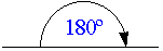
To illustrate the principles behind accelerated testing, consider the following simple example which involves a paper clip and can be easily and independently performed by the reader. The objective was to determine the mean number of cycles-to-failure of a given paper clip. The use cycles were assumed to be at a 45º bend. The acceleration stress was determined to be the angle to which we bend the clips, thus two accelerated bend stresses of 90º and 180º were used. The paper clips were tested using the following procedure for the 90º bend. A similar procedure was also used for the 180º and 45º test.

1) Open the Paper Clip.

2) With one hand, hold the clip by the longer, outer loop.

3) With the thumb and forefinger of the other hand, grasp the smaller, inner loop.

4) Pull the smaller, inner loop out and down 90 degrees so that a right angle is formed as shown.

5) Close the Paper Clip.

6) With one hand, continue to hold the clip by the longer, outer loop.

7) With the thumb and forefinger of the other hand, grasp the smaller, inner loop.

8) Push the smaller inner loop up and in 90 degrees so that the smaller loop is returned to the original upright position in line with the larger, outer loop as shown.

9) This completes one cycle.

10) Repeat until the paper clip breaks. Count and record the cycles-to-failure for each clip.

At this point, the reader must note that the paper clips used in this example were Jumbo paper clips capable of repeated bending. Different paper clips will yield different results. Additionally, and so that no other stresses are imposed, caution must be taken to assure that the rate at which the paper clips are cycled remains the same across the experiment.

For the experiment, a sample of six paper clips was tested to failure at both 90º and 180º bends. A base test sample of six paper clips was tested at a 45º bend (the assumed use stress level) to confirm the analysis. The cycles-to-failure are given next.

Cycles-to-Failure at [math]\displaystyle{ 90^\circ }[/math]

Cycles-to-Failure at [math]\displaystyle{ 180^\circ }[/math]

Cycles-to-Failure at [math]\displaystyle{ 45^\circ }[/math]

The accelerated test data set was then analyzed in ALTA, assuming a lognormal life distribution (fatigue) and an inverse power law relationship (non-thermal) for the life-stress model. The analysis and some of the results are shown in Figs. 1, 2, 3 and 4 next. Fig. 5 shows the analysis of the base data in Weibull++ and the base MTTF estimate. In this case, our accelerated test correctly predicted the MTTF as verified by our base test.

Fig. 1: The accelerated test data analyzed in ALTA.

Fig. 2: Lognormal probabiliyt plot of both stress levels from ALTA.

Fig. 3: The resulting Acceleration Factor vs. Stress plot from ALTA.

Fig 4

Fig. 5: The base [math]\displaystyle{ 45^\circ }[/math] data analyzed in ReliaSoft's Weibull++, utilizing a lognormal distribution shown on lognormal probability paper, along with the MTTF estimate of 70.45 cycles from the QCP.

Example 2

Twelve electronic devices were put into a continuous accelerated test. The accelerated stresses were temperature and voltage, with use level conditions of 328K and 2V respectively. The data set obtained is shown in the table below:

Do the following:

1) Using the T-NT Weibull model, analyze the data in ALTA and determine the MTTF and .. life for these devices at use level. Determine the upper and lower 90% 2-sided confidence intervals on the results.

2) Examine the effects of each stress on life.

Solution to Example 2

The data set was analyzed in ALTA and the following MTTF and [math]\displaystyle{ B(10) }[/math] life results were obtained: (The results are shown in ALTA's QCP in the following figures.)

• Figs. 6 and 7 examine the effects of each stress on life, while Fig. 8 examines the effects of the combined stresses on the reliability. Specifically, Fig. 6 below shows the Life vs. Voltage plot with temperature held constant at 328K.

Fig. 6: The effects of voltage on life, with temperature held constant.

Fig. 7 below shows the Life vs. Temperature plot with voltage held constant at 2V.

Fig. 7: The effects of temperature on life, with voltage held constant.

Fig. 8 below shows a 3D plot of reliability (at a constant time) versus both stresses. One can observe that reliability declines slightly faster with the change in temperature than with the change in voltage. Note that in the following plot, Stress 1 refers to temperature and Stress 2 refers to voltage.

Fig. 8: The combined effects of voltage and temperature on the reliability, as plotted in ALTA.

Example 3

A mechanical component was put into an accelerated test with temperature as the accelerated stress. The following times-to-failure were observed.

343 K	363 K	383 K
266.66	618.54	351.12
430.09	666.72	355.1
570.45	724.4	672.69
890.42	950.89	923.35
1046.65	1148.4	948.22
1158.14	1202.94	1277.04
1396.01	1492.56	1538.81
1918.38	1619.59	2020.34
2028.86	2592.29	2099.03
2785.58	3596.85	2173.04

1) Determine the parameters of the Arrhenius-Weibull model.

2) What is your observation?

Solution to Example 3

The parameters of the Arrhenius Weibull model were estimated using ALTA with the following results:

[math]\displaystyle{ \beta =1.771456,\text{ }B=86.273322,\text{ }C=1170.142567. }[/math]

A small value for [math]\displaystyle{ B }[/math] was estimated. The following observations can then be made:

• Life is not accelerated with temperature, or
• the stress increments were not sufficient, or
• the test stresses were well within the ``specification limits for the product (see discussion in Chapter 2, Section 2.2.3).

A small value for [math]\displaystyle{ B }[/math] is not the only indication for this behavior. One can also observe from the data that at all three stress levels, the times-to-failure are within the same range. Another way to observe this is by looking at the Arrhenius plot. The scale parameter, [math]\displaystyle{ \eta }[/math] , and the mean life are plotted next.

Fig 9: Eta and Mean Life vs. Stress.

It can be seen that life ( [math]\displaystyle{ \eta }[/math] , and the mean life) is almost invariant with stress.

Example 4

A tensile component of a landing gear was put through an accelerated reliability test to determine whether the life goal would be achieved under the designed-in load. Fifteen units, N=15, were tested at three different shock loads. The component was designed for a peak shock load of 50 kips with an estimated return of 10% of the population by 10,000 landings. Using the inverse power law lognormal model, determine whether the design life was met.

Failure, in Cycles	Shock Load, kips
1855	73
2158	73
2425	73
2736	73
3206	73
614	95
770	95
781	95
890	95
1055	95
152	128
162	128
173	128
209	128
216	128

Solution to Example 4

The data were entered into ALTA, and the following estimates were obtained for the parameters of the IPL-lognormal model:

- [math]\displaystyle{ \begin{align} - & Std= & 0.179080 \\ - & K= & 8.953055E-13 \\ - & n= & 4.638882 - \end{align} }[/math]

The probability plot at each test stress level (73 kips, 95 kips and 123 kips) was then obtained, as shown next.

Fig. 10: Probability plots at different shock loads.

In this plot, it can be seen that there is a good agreement between the data and the fitted model. The probability plot at a use stress level of 50 kips is shown next.

Fig. 11: The probability plot at a use stress level of 50 kips.

Using the Use Level Probability plot, the cycles-to failure for a 10% probability of failure can be estimated. From the plot, this time is estimated to be [math]\displaystyle{ T(Q=0.10=10%)\approxeq 12,000 }[/math] landings. Another way to obtain life information is by using a Life vs. Stress plot. Once a Life vs. Stress plot is selected, the 10% unreliability (probability of failure) line must be plotted. To do this, click Life Lines... in the plot panel and and select the 10% Unreliability box (or enter 10 in one of the boxes and select the box) in the Specify Life Lines window, as shown next.

In the following plot, the 10% unreliability line is plotted (the first line from the left). For a stress of 50 psi (X-axis) and for the 10% unreliability line, the cycles-to-failure can be obtained by reading the value on the Y-axis. Again, [math]\displaystyle{ T(0.1)\approxeq 12,000 }[/math] landings.

Fig. 12: Mean Lif line (left) and 10% unreliability line (right) vs. stress.

However, a more accurate way to obtain such information is by using the Quick Calculation Pad (QCP) in ALTA. Using the QCP, the life for a 10% probability of failure at 50 kips is estimated to be 11,668.73 cycles (or landings), as shown next.

The design criterion of 10,000 landings is met.

Example 5

In the previous example, it was found that the 10,000 landings life criterion for a 90% reliability was met. However, the estimate of 11,668.73 cycles (or landings) is very close to the requirement. Additionally, this estimate was obtained at the 50% confidence level. In other words, 50% of the time life will be greater than 10,544.899 landings, and 50% of the time life will be less. A lower confidence level is thus crucial before any decisions are made. Repeat the calculation of the previous example, and this time include a 90% lower 1-sided confidence bound on the estimation.

Solution to Example 5

Using ALTA's QCP, the 90% lower 1-sided confidence bound on the 11,668.73 cycles-to-failure can be obtained.

The 90% lower 1-sided confidence bound is estimated to be 9,680.51 landings. Thus the 10,000 landings criterion is not quite met.

Example 6

ACME manufacturing has implemented an accelerated testing program for their new design. A total of 40 units were tested at four different pressure levels. The operating stress level is 170 psi.

Stress Level, psi	220 psi	230 psi	240 psi	250 psi
	165	93	72	26
	177	106	73	44
	238	156	99	63
	290	170	124	68
Times-to-failure, hr	320	185	134	69
	340	214	150	72
	341	220	182	77
	380	236	186	96
	449	252	190	131
	544	288	228	140

Do the following:

1) Determine the parameters of the inverse power law Weibull model.

2) Obtain the use level probability plot with 90% 2-sided confidence bounds on time.

3) Obtain the Life vs. Stress plot with 90% 2-sided confidence bounds.

Solution to Example 6

1) The parameters of the IPL-Weibull model are estimated to be:

- [math]\displaystyle{ \begin{align} - & \beta = & 3.009236 \\ - & K= & 3.267923E-27 \\ - & n= & 10.218104 - \end{align} }[/math]

2) The use level probability plot is shown next.

Fig. 13: The probability plot at a use stress level.

The confidence bounds on time are the Type 1 bounds (Time Bounds) in ALTA.

Fig. 14: The probability plot at a use stress level with 90% Type I confidence bounds.

3)Similarly, the Life vs. Stress plot with the confidence bounds can be obtained.

Example 7

Twenty-seven circuit boards were tested with temperature as the accelerated stress (or stimuli). The goal was to estimate the reliability after 10 years at 100ºC. The circuit boards were tested and the following data obtained:

[math]\displaystyle{ }[/math]

The data were entered in ALTA and analyzed utilizing an Arrhenius-Weibull model. Note that all units that did not fail in the test but failed for unrelated reasons were entered as suspensions. The plot that follows shows the predicted reliability after 10 years at 100ºC.

Example 8

An electronic component was redesigned and was tested to failure at three different temperatures. Six units were tested at each stress level. At the 406K stress level however, a unit was removed from the test due to a test equipment failure which led to a failure of the component. A warranty time of one year is to be given, with an expected return of 10% of the population. The times-to-failure and test temperatures are given next:

The operating temperature is 356K. Using the Arrhenius-Weibull model, determine the following:

1) Should the first failure at 406K be included in the analysis?

2) Determine the warranty time for a 90% reliability.

3) Determine the 90% lower confidence limit on the warranty time.

4) Is the warranty requirement met? If not, what steps should be taken?

5) Repeat the analysis with the unrelated failure included. Is there any difference?

6) If the unrelated failure occurred at 500 hr, should it be included in the analysis?

Solution to Example 8

1) Since the failure occurred at the very beginning of the test and for an unrelated reason, it can be omitted from the analysis. If it is included it should be treated as a suspension and not as a failure.

2) The first failure at 406K was neglected and the data were analyzed using ALTA. The following parameters were obtained:

[math]\displaystyle{ \begin{align} & \beta = & 2.9658 \\ & B= & 10679.57 \\ & C= & 2.39662\cdot {{10}^{-9}} \end{align} }[/math]

The use level probability plot (at 356K) can then be obtained. The warranty time for a reliability of 90% (or an unreliability of 10%) can be estimated from this plot as shown next.

Fig. 16: The probability plot at use stress level.

This estimate can also be obtained from the Arrhenius plot (a Life vs. Stress plot). The 10th percentile (time for a reliability of 90%) is plotted versus stress. This type of plot is useful because a time for a given reliability can be determined for different stress levels.

Fig. 17: 10% unreliability vs stress.

A more accurate way to determine the warranty time would be to use ALTA's Quick Calculation Pad (QCP). By selecting the Warranty (Time) Information option from the Basic Calculations tab in the QCP and entering 356 for the temperature and 90 for the required reliability, a warranty time of 11,977.793 hr can be determined, as shown next:

3) The warranty time for a 90% reliability was estimated to be approximately 12,000 hr. This is above the 1 year (8,760 hr) requirement. However, this is an estimate at the 50% confidence level. In other words, 50% of the time life will be greater than 12,000 hr and 50% of the time life will be less. A known confidence level is therefore crucial before any decisions are made. Using ALTA, confidence bounds can be plotted on both probability and Arrhenius plots. In the following use level probability plot, the 90% lower confidence level (LCL) is plotted. Note that percentile bounds are Type 1 confidence bounds in ALTA.

Fig. 18: The use level probability plot with the Type I 90% lower bound.

An estimated 4,300 hr warranty time at a 90% lower confidence level was obtained from the use level probability plot. This means that 90% of the time, life will be greater than this value. In other words, a life of 4,300 hr is a bounding value for the warranty.

Fig. 19: Life vs Stress plot with the 90% lower confidence level.

The Arrhenius plot with the 90% lower confidence level is shown next.

Using the QCP and specifying a 90% lower confidence level, a warranty time of 4436.5 hr is estimated, as shown next.

4)The warranty time for this component is estimated to be 4,436.5 hr at a 90% lower confidence bound. This is much less than the 1 year warranty time required (almost 6 months). Thus the desired warranty is not met. In this case, the following four options are available:

a) Redesign.

b) Reduce the confidence level.

c) Change the warranty policy.

d) Test additional units at stress levels closer to the use level.

Including the unrelated failure of 0.3 hr at 406 K (by treating it as a suspension at that time), the following results are obtained:

- [math]\displaystyle{ \begin{align} - & \beta = & 2.9658 \\ - & B= & 10679.57 \\ - & C= & 2.39662\cdot {{10}^{-9}} - \end{align} }[/math]

These results are identical to the ones with the unrelated failure excluded. A small difference can be seen only if more significant digits are considered. The warranty time with the 90% lower 1-sided confidence bound was estimated to be:

- [math]\displaystyle{ \begin{align} - & T= & 11977.729\text{ hr} \\ - & {{T}_{L}}= & 4436.46\text{ hr} - \end{align} }[/math]

Again, the difference is negligible. This is due to the very early time at which this unrelated failure occurred.

The analysis is repeated treating the unrelated failure at 500 hr as a suspension, with the following results:

- [math]\displaystyle{ \begin{align} - & \beta = & 3.0227 \\ - & B= & 10959.52 \\ - & C= & 1.23808\cdot {{10}^{-9}} - \end{align} }[/math]

In this case, the results are very different. The warranty time with the 90% lower 1-sided confidence bound is estimated to be:

[math]\displaystyle{ \begin{align} & T= & 13780.208\text{ hr} \\ & {{T}_{L}}= & 5303.67\text{ hr} \end{align} }[/math]

It can be seen that in this case, it would be a mistake to neglect the unrelated failure. By neglecting this failure, we would actually underestimate the warranty time. The important observation in this example is that every piece of life information is crucial. In other words, unrelated failures also provide information about the life of the product. An unrelated failure occurring at 500 hr indicates that the product has survived for that period of time under the particular stress level, thus neglecting it would be a mistake. On the other hand it would also be a mistake to treat this data point as a failure, since the failure was caused by a test equipment failure.

Example 9

An electronic component was subjected to a voltage stress, starting at 2V (use stress level) and increased to 7V in stepwise increments. The following steps, in hours, were used to apply stress to the products under test: 0 to 250, 2V; 250 to 350, 3V; 350 to 370, 4V; 370 to 380, 5V; 380 to 390, 6V; and 390 to 400, 7V. This profile is represented graphically next.

The objective of this test was to determine the [math]\displaystyle{ B10 }[/math] life of these components at the normal use stress level of 2V.
In this experiment, the overall test time was 385 hrs. If the test had been performed at use conditions, one would expect the test duration to be approximately 1700 hrs if the test were run until all units failed.
Eleven units were available for the test. All eleven units were tested using the same stress profile. Units that failed were removed from the test and their total time on test recorded. The following times-to-failure were observed in the test, in hours: 280, 310, 330, 352, 360, 366, 371, 374, 378, 381 and 385.

Solution to Example 9

After creating a Standard Folio for a single stress (voltage), the analyst used the Add Stress Profile option in the Project menu to create the stress profile for this experiment.
In ALTA's stress profile, you can define any stress profile in segments. The stress applied during these segments can be a constant value (as is the case in this step example) or defined as a function of a time variable (t). The stress profile for this analysis is displayed next.

Fig. 21: The voltage test profile as in ALTA.

The times-to-failure data are entered in the ALTA Standard Folio with the following analysis options selected: cumulative damage power life-stress relationship and Weibull for the underlying life distribution. The ALTA Standard Folio with the data entered and the estimated parameters is shown next. Notice that the voltage step-stress profile has been assigned to each data point.

The [math]\displaystyle{ B10 }[/math] life at the 2V use stress level, can be calculated with ALTA's Quick Calculation Pad (QCP), as shown next.

Example 10

Consider a test in which multiple stresses were applied simultaneously to a particular automotive part in order to precipitate failures more quickly than they would occur under normal use conditions. The engineers responsible for the test were able to quantify the combination of applied stresses in terms of a ``percentage stress as compared to typical stress levels (or assumed field conditions). In this scenario, the typical stress (field or use stress) was defined as 100% and any combination of the test stresses was quantified as a percentage over the typical stress. For example, if the combination of stresses on test was determined to be two times higher than typical conditions, then the stress on test was said to be at 200%. The test was set up and run as a step-stress test (i.e. the stresses were increased in a stepwise fashion) and the time on test was measured in hours. The step-stress profile used was as follows: until 200 hours, the equivalent applied stress was 125%; from 200 to 300 hrs, it was 175%; from 300 to 350 hrs, it was 200% and from 350 to 375 hrs, it was 250%. The test was terminated after 375 hours and any units that were still running after that point were right-censored (suspended). Additionally, and based on prior analysis/knowledge, the engineers also stated that each hour on test under normal use conditions (i.e., at 100% stress measure) was equivalent to approximately 100 miles of normal driving. The test was conducted and the following times-to-failure and times-to-suspension under the stated step-stress profile were observed (note that XXX+ indicates a non-failed unit, i.e., suspension): 252, 280, 320, 328, 335, 354, 361, 362, 368, 375+, 375+, 375+. After performing failure analysis on the failed parts, it was determined that the failure that occurred at 328 hrs was due to mechanisms other than the ones considered. That data point was therefore identified as a suspension in the currently analysis. The modified data set for this analysis was: 252, 280, 320, 328+, 335, 354, 361, 362, 368, 375+, 375+, 375+.

The test objective was to estimate the [math]\displaystyle{ B1 }[/math] life for the part (i.e. time at which reliability is equal to 99%) at the typical operating conditions (i.e., Stress=100%), in miles.

Solution to Example 10

Utilizing ALTA PRO, the analyst first created a Standard Folio for non-grouped time-to-failure and time-to-suspension data and used the Add Stress Profile from the Project menue to define the stress profile, as shown next.

Once the profile was defined, the analyst entered the observed times, their state (i.e., failed F or non-failed S) and a reference to the profile used in the ALTA Standard Folio. The analyst selected the cumulative damage life-stress relationship (to use a time-varying stress) based on a power model (since the effect of the stress was deemed to be mechanical and more appropriately modeled by a power function). The Weibull distribution was selected as the underlying life distribution. Additionally, note that the use stress was set to 100 and all results were then extrapolated to the typical stress level. The Standard Folio and the selected model is shown next.

The estimated parameters are shown next.

The last part remaining was to determine the [math]\displaystyle{ B1 }[/math] life at the part's use stress level. Using the QCP, the [math]\displaystyle{ B1 }[/math] life was found to be 658 hours, as shown next.

Based on the given multiplier, the [math]\displaystyle{ B1 }[/math] life in miles would then be 658 test-hr*100 (miles/test-hr)= 65,800 miles.

The [math]\displaystyle{ B1 }[/math] life can also be obtained from the use level probability plot, as shown next.

Example 11

A sample of and electronic device was tested in two testing chambers set at different temperatures and monitored on a weekly basis. The test was perfromed continously for 15 weeks. 50 units were put in each chamber. The goal of the test is to estimate the 90% lower bound on the [math]\displaystyle{ B10 }[/math] life (in hours) of the electronic device. The following figure represents the test results, it shows the test results entered in ALTA in an interval data format. The normal use condition is assumed to be 300K.

Solution to Example 11

Assuming that the failure times of the devices follow a Weibull distribution and that the Arrhenius model is an adequate life-stress relationship, we obtain the followingestimated model parameters:

[math]\displaystyle{ \begin{align} & \beta = & 3.4259 \\ & B= & 1488.4127 \\ & C= & 24.0596 \end{align} }[/math]

The next figure show the probabilty lines at the differnet stress levels along with the extrapolated use level probability line.

Fig. 22: Probabilty lines at the different test stress levels with the extrapolated use level probability line.

The following is the life versus stress plot showing the [math]\displaystyle{ B10 }[/math] life line.

Fig. 32: Life vs. Stress with the B10 life line (bottom).

The 90% lower bound on the [math]\displaystyle{ B10 }[/math] life can be estimated as follows.

[math]\displaystyle{ }[/math]