Growth Plan for Three Phases
 |
New format available! This reference is now available in a new format that offers faster page load, improved display for calculations and images and more targeted search.
As of January 2024, this Reliawiki page will not continue to be updated. Please update all links and bookmarks to the latest references at RGA examples and RGA reference examples.
This example appears in the Reliability growth reference.
A complex system is under design. The reliability team wants to create an overall reliability growth plan based on the Crow Extended model. The inputs to the model are the following:
- The requirement or goal MTBF is [math]\displaystyle{ {{M}_{G}}=56\,\! }[/math] hours.
- The growth potential design margin factor is [math]\displaystyle{ GPDM=1.35\,\! }[/math].
- The average effectiveness factor is [math]\displaystyle{ d\quad =0.7.\,\! }[/math]
- The management strategy is [math]\displaystyle{ msr=0.95\,\! }[/math].
- The beta parameter for the discovery function, [math]\displaystyle{ h\left( t \right),\,\! }[/math] of the type B failure modes is [math]\displaystyle{ \beta =0.7.\,\! }[/math]
- The test will be conducted in three phases. The cumulative phase end times are [math]\displaystyle{ {{T}_{1}}=1500,{{T}_{2}}=3500\,\! }[/math] and [math]\displaystyle{ {{T}_{3}}=4500\,\! }[/math] hours. The average fix delays for each phase are [math]\displaystyle{ {{L}_{1}}=500\,\! }[/math], [math]\displaystyle{ {{L}_{2}}=700\,\! }[/math] and [math]\displaystyle{ {{L}_{3}}=1000\,\! }[/math] test hours, respectively.
Determine the following:
- The growth potential MTBF and failure intensity.
- The initial failure intensity.
- The type A and type B initial failure intensity.
- The parameter [math]\displaystyle{ \lambda \,\! }[/math] of the Crow extended model.
- The type B failure mode discovery function.
- The initialization time, [math]\displaystyle{ {{t}_{0}},\,\! }[/math] for the nominal failure intensity function.
- The nominal idealized failure intensity function.
- The nominal time to reach the MTBF goal.
- The MTBF that can be reached at the end of the last test phase based on the nominal idealized growth curve.
- The actual initialization time for phase 1, [math]\displaystyle{ T_{0}^{AIC}.\,\! }[/math]
- The MTBF that can be reached at the end of the last test phase based on the actual idealized growth curve.
- The actual time to reach the MTBF goal.
- The actual time to reach the MTBF goal if the cumulative end phase time for the third (last) phase is [math]\displaystyle{ {{T}_{3}}=6000\,\! }[/math] hours.
- Use the RGA software to generate the results for this example. Consider the cumulative last phase as [math]\displaystyle{ {{T}_{3}}=6000\,\! }[/math] hours, as given in question 13.
Solution
- The growth potential MTBF is:
- [math]\displaystyle{ \begin{align} {{M}_{GP}}= & GPDM\cdot M_{G} \\ = & 56\cdot 1.35 \\ = & 75.6 \end{align}\,\! }[/math]
- [math]\displaystyle{ \begin{align} {{\lambda }_{GP}}= & \frac{1}{{{M}_{GP}}} \\ = & \frac{1}{75.6} \\ = & 0.0132 \end{align}\,\! }[/math]
- The initial failure intensity is given by:
- [math]\displaystyle{ \begin{align} {{\lambda }_{I}}= & \frac{{{\lambda }_{GP}}}{1-d\cdot msr} \\ = & \frac{0.0132}{\left( 1-0.7\cdot 0.95 \right)} \\ = & 0.0394 \end{align}\,\! }[/math]
- The type A failure mode intensity, [math]\displaystyle{ {{\lambda }_{A}},\,\! }[/math] is:
- [math]\displaystyle{ \begin{align} \lambda_{A}=&(1-msr)\lambda_{I} \\ =& (1-0.95)0.375 \\ =& 0.0019 \end{align}\,\! }[/math]
- [math]\displaystyle{ \begin{align} {{\lambda }_{B}}= & msr\cdot {{\lambda }_{I}} \\ = & 0.95\cdot 0.0394 \\ = & 0.0375 \end{align}\,\! }[/math]
- Using the inputs of [math]\displaystyle{ {{\lambda }_{B}}\,\! }[/math] and [math]\displaystyle{ \beta \,\! }[/math] in the failure intensity equation for the Crow-AMSAA (NHPP) model, we have:
- [math]\displaystyle{ 0.0375=\frac{{{\lambda }^{\left( \tfrac{1}{0.7} \right)}}}{\Gamma \left( 1+\tfrac{1}{0.7} \right)}\,\! }[/math]
- [math]\displaystyle{ 0.0375=\frac{{{\lambda }^{1.428}}}{1.2658}\,\! }[/math]
- [math]\displaystyle{ \begin{align} \lambda = & {{\left( 0.0375\cdot 1.2658 \right)}^{\left( \tfrac{1}{1.428} \right)}} \\ = & 0.1184 \end{align}\,\! }[/math]
- The type B failure mode discovery function is:
- [math]\displaystyle{ h\left( t \right)=\lambda \beta {{t}^{\beta -1}}\,\! }[/math]
- [math]\displaystyle{ \begin{align} h\left( t \right)= & 0.1183\cdot 0.7{{t}^{0.7-1}} \\ = & 0.0828{{t}^{-0.3}} \end{align}\,\! }[/math]
- The initialization time, [math]\displaystyle{ {{t}_{0}},\,\! }[/math] is:
- [math]\displaystyle{ \begin{align} {{t}_{0}}= & {{\left[ \frac{{{\lambda }_{I}}-{{\lambda }_{A}}-(1-d){{\lambda }_{B}}}{d\lambda \beta } \right]}^{\tfrac{1}{\beta -1}}} \\ = & {{\left[ \frac{0.0394-0.001974-(1-0.7)0.0375}{0.7\cdot 0.1183\cdot 0.7} \right]}^{\tfrac{1}{0.7-1}}} \end{align}\,\! }[/math]
- [math]\displaystyle{ \begin{align} {{t}_{0}}=14.07 \end{align}\,\! }[/math]
- The nominal idealized growth curve is given by the following equation:
- [math]\displaystyle{ {{r}_{NI}}\left( t \right)=\left\{ \begin{matrix} {{\lambda }_{I}} & t\le {{t}_{0}} \\ \begin{matrix} {{r}_{IT}}(t)={{\lambda }_{A}}+(1-d){{\lambda }_{B}}+d\lambda \beta {{t}^{\left( \beta -1 \right)}} \\ \end{matrix} & t\gt {{t}_{0}} \\ \end{matrix} \right\}\,\! }[/math]
- [math]\displaystyle{ {{r}_{NI}}\left( t \right)=\left\{ \begin{matrix} 0.0394 & t\le 14.07 \\ =0.0013+0.058\cdot {{t}^{-0.3}} & t\gt 14.07 \\ \end{matrix} \right\}\,\! }[/math]
- The nominal time to reach the MTBF goal is:
- [math]\displaystyle{ {{t}_{N,goal}}={{\left[ \frac{{{r}_{G}}-{{\lambda }_{A}}-(1-d){{\lambda }_{B}}}{d\lambda \beta } \right]}^{\tfrac{1}{\beta -1}}}\,\! }[/math]
- [math]\displaystyle{ \begin{align} {{r}_{G}}= & \frac{1}{{{M}_{G}}} \\ = & \frac{1}{56} \\ = & 0.01785 \end{align}\,\! }[/math]
- [math]\displaystyle{ \begin{align} {{t}_{N,G}}= & {{\left[ \frac{0.01785-0.001974-(1-0.7)0.0375}{0.7\cdot 0.1184\cdot 0.7} \right]}^{^{\tfrac{1}{\beta -1}}}} \\ = & 4578\text{ hours} \end{align}\,\! }[/math]
- Using the equation for the nominal failure intensity, we find the failure intensity that can be reached at the end of the last test phase based on the nominal idealized growth curve, [math]\displaystyle{ {{r}_{NI,final}}\,\! }[/math]. The total (cumulative) test time is [math]\displaystyle{ T=4500\,\! }[/math] hours. Therefore we have:
- [math]\displaystyle{ \begin{align} {{r}_{NI,final}}= & {{\lambda }_{A}}+(1-d){{\lambda }_{B}}+d\lambda \beta {{T}^{\left( \beta -1 \right)}}\text{ } \\ = & 0.0019+\left( 1-0.7 \right)0.0375+0.7\cdot 0.1184\cdot 0.7\cdot {{(4500)}^{0.7-1}} \\ = & 0.01788 \end{align}\,\! }[/math]
- [math]\displaystyle{ \begin{align} {{M}_{NI,final}}= & \frac{1}{{{r}_{NI,final}}} \\ = & \frac{1}{0.01788} \\ = & 55.92 \end{align}\,\! }[/math]
- We can find the actual initialization time by using:
- [math]\displaystyle{ T_{0}^{AIC}=\frac{{{t}_{0}}}{\left( \tfrac{{{T}_{1}}-{{L}_{1}}}{{{T}_{1}}} \right)}\,\! }[/math]
- [math]\displaystyle{ \begin{align} T_{0}^{AIC}= & \frac{14.07}{\left( \tfrac{1500-500}{1500} \right)} \\ = & 21.10887 \end{align}\,\! }[/math]
- The failure intensity that can be reached at the end of the last test phase based on the actual idealized growth curve for [math]\displaystyle{ T=4500\,\! }[/math] hours is given by:
- [math]\displaystyle{ \begin{align} {{r}_{AI,final}}(T)= & {{\lambda }_{A}}+(1-d){{\lambda }_{B}} \\ & +d\lambda \beta {{\left[ {{T}_{2}}-{{L}_{2}}+\left( \frac{{{T}_{3}}-{{L}_{3}}-{{T}_{2}}+{{L}_{2}}}{{{T}_{3}}-{{T}_{2}}} \right)(T-{{T}_{2}}) \right]}^{(\beta -1)}} \end{align}\,\! }[/math]
- [math]\displaystyle{ \begin{align} {{r}_{AI,final}}(T)= & 0.0019+\left( 1-0.7 \right)0.0375+0.7\cdot 0.1184\cdot 0.7 \\ & \cdot {{\left[ 3500-700+\left( \frac{4500-1000-3500+700}{4500-3500} \right)(4500-3500) \right]}^{(0.7-1)}} \end{align}\,\! }[/math]
- [math]\displaystyle{ \begin{align} {{r}_{AI,final}}(T)=0.0182 \end{align}\,\! }[/math]
- [math]\displaystyle{ \begin{align} {{M}_{AI,final}}= & \frac{1}{{{r}_{AI,final}}} \\ = & \frac{1}{0.0182} \\ = & 54.80 \end{align}\,\! }[/math]
- From question 11, it is shown that the actual final MTBF that can be reached at 4,500 hours of test time is less than the MTBF goal for the program. So, in accordance with the third case that is described in Actual Time to Reach Goal section, this is the scenario where the actual time to meet the MTBF goal will not be calculated since the reliability growth program needs to be redesigned.
- The failure intensity that can be reached at the end of the last test phase based on the actual idealized growth curve for [math]\displaystyle{ T={{T}_{3}}=6000\,\! }[/math] hours is given by:
- [math]\displaystyle{ \begin{align} {{r}_{AI,final}}(T)= & {{\lambda }_{A}}+(1-d){{\lambda }_{B}} \\ & +d\lambda \beta {{\left[ {{T}_{2}}-{{L}_{2}}+\left( \frac{{{T}_{3}}-{{L}_{3}}-{{T}_{2}}+{{L}_{2}}}{{{T}_{3}}-{{T}_{2}}} \right)(T-{{T}_{2}}) \right]}^{(\beta -1)}} \end{align}\,\! }[/math]
- [math]\displaystyle{ \begin{align} {{r}_{AI,final}}(T)= & 0.0019+\left( 1-0.7 \right)0.0375+0.7\cdot 0.1184\cdot 0.7 \\ & \cdot {{\left[ 3500-700+\left( \frac{6000-1000-3500+700}{6000-3500} \right)(6000-3500) \right]}^{(0.7-1)}} \end{align}\,\! }[/math]
- [math]\displaystyle{ \begin{align} {{r}_{AI,final}}(T)=0.0177 \end{align}\,\! }[/math]
- [math]\displaystyle{ \begin{align} {{M}_{AI,final}}= & \frac{1}{{{r}_{AI,final}}} \\ = & \frac{1}{0.0177} \\ = & 56.38 \end{align}\,\! }[/math]
- [math]\displaystyle{ {{t}_{AC,G}}=\frac{{{t}_{N,G}}-{{T}_{F-1}}+{{L}_{F-1}}}{\left( \tfrac{{{T}_{F}}-{{L}_{F}}-{{T}_{F-1}}+{{L}_{F-1}}}{{{T}_{F}}-{{T}_{F-1}}} \right)}+{{T}_{F-1}}\,\! }[/math]
- [math]\displaystyle{ {{t}_{AC,G}}=\frac{4578-3500+700}{\left( \tfrac{6000-1000-3500+700}{6000-3500} \right)}+3500\,\! }[/math]
- [math]\displaystyle{ \begin{align} {{t}_{AC,G}}=5521 \end{align}\,\! }[/math]
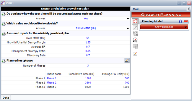
- To use RGA to obtain the results for this example, first we create a growth planning folio by choosing Insert > Test and Planning > Continuous Growth Planning. In the growth planning folio, specify the number of phases, the cumulative phase time and average fix delays for each of the three phases, as shown in the figure below.
We then enter the remaining input needed by the Crow Extended model, as shown in the following figure.
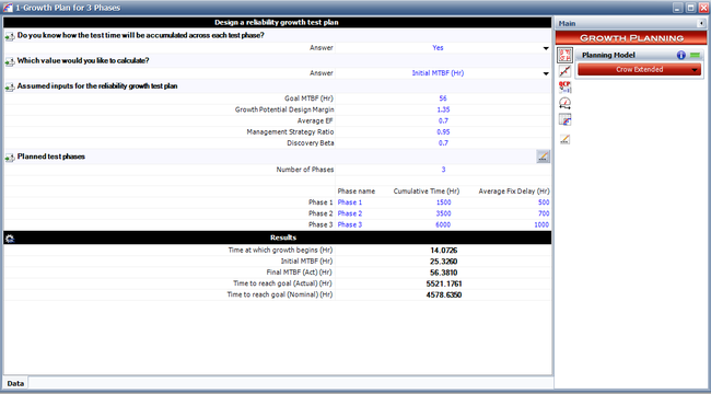
The input provided is the required MTBF goal of 56, the growth potential design margin of 1.35, the management strategy of 0.95 and the discovery beta of 0.7. The results show the initialization time, [math]\displaystyle{ {{t}_{o}}\,\! }[/math], the initial MTBF, the final actual MTBF that can be reached for this growth program and the actual time when the MTBF goal is met. Note that in this case we provided the goal MTBF and solved for the initial MTBF.
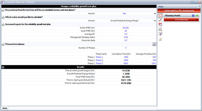
Different calculation options are available depending on the desired input and output. For example, we could provide the initial and goal MTBF to solve for the growth potential design margin, as shown in the figure below.
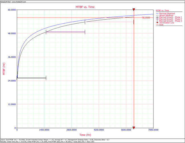
Click the Plot icon to generate a plot that shows the nominal and actual idealized growth curve, the test termination time, the MTBF goal and the planned growth for each phase, as shown in the figure below.