Markov Diagrams

The term "Markov Chain," invented by Russian mathematician Andrey Markov, is used across many applications to represent a stochastic process made up of a sequence of random variables representing the evolution of a system. Events are "chained" or "linked" serially together though memoryless transitions from one state to another. The term "memoryless" is used because past events are forgotten, as they are irrelevant; an event or state is dependent only on the state or event that immediately preceded it.

Concept and Methodology

The concept behind the Markov chain method is that given a system of states with transitions between them, the analysis will give the probability of being in a particular state at a particular time. If some of the states are considered to be unavailable states for the system, then availability/reliability analysis can be performed for the system as a whole.

Depending on the transitions between the states, the Markov chain can be considered to be a discrete Markov chain, which has a constant probability of transition per unit step, or a continuous Markov chain, which has a constant rate of transition per unit time.

Discrete Markov Chains

A discrete Markov chain can be viewed as a Markov chain where at the end of a step, the system will transition to another state (or remain in the current state), based on fixed probabilities. It is common to use discrete Markov chains when analyzing problems involving general probabilities, genetics, physics, etc. To represent all the states that the system can occupy, we can use a vector ▁X:

▁X(0)=(■(X_1&X_2&⋯&X_i ))

where the term X_i represents the probability of the system being in state i and with:

∑_(i=1)^n▒X_i =1

The transitions between the states can be represented by a matrix ▁P:

▁P=(■(P_11&P_12&⋯&P_1i@P_21&P_22&⋯&P_2i@⋮&⋮&⋱&⋮@P_i1&P_i2&⋯&P_ii ))

where, for example, the term P_12 is the transition probability from state 1 to state 2, and for any row m with i states:

∑_(j=1)^i▒P_mj =1

To determine the probability of the system being in a particular state after the first step, we have to multiply the initial state probability vector ▁X(0) with the transition matrix ▁P:

▁X (1)=▁X(0)∙▁P

This will give us the state probability vector after the first step, ▁X(1).

If one wants to determine the probabilities of the system being in a particular state after n steps, the Chapman-Kolmogorov equation can be used. This equation states that the probabilities of being in a state after n steps can be calculated by taking the initial state vector and multiplying by the transition matrix to the nth power, or:

▁X (n)=▁X (0)∙▁P^n

Example

Take a system that can be in any one of three states-- operational, standby or offline-- at a given time, and starts in the standby state.

After each step:

• If the system is in the operational state, there is a 20% chance that it moves to the standby state, and a 5% chance that it goes offline.
• If it is in the standby state, there is a 40% chance that it becomes operational, and a 1% chance that it goes offline.
• If it is in the offline state, there is a 15% chance that it becomes operational, and a 50% chance that it moves to the standby state.

We want to know the probability that it is offline after 10 steps.

First, we must create the state probability vector at time equal to zero, which in this case is:

▁X(0)=(■(0&1&0))

Then, we can create the transition matrix to represent all the various transition probabilities between states:

▁P=(■(0.75&0.20&[email protected]&0.59&[email protected]&0.50&0.35))

Lastly, we can calculate the state probabilities after 10 steps using the Chapman-Kolmogorov equation:

▁X (10)=▁X (0)∙▁P^10

or:

▁X (10)=(■(0&1&0))∙(■(0.75&0.20&[email protected]&0.59&[email protected]&0.50&0.35))^10

resulting in :

▁X (10)=(■(0.596&0.353&0.051))

We can also plot the point probabilities of each state at each step if we calculate the state probabilities after each step:

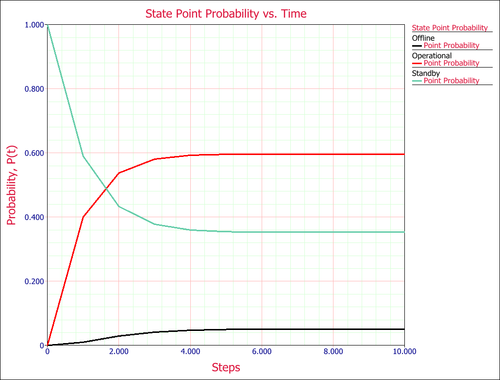
From the plot, we can also determine that the probabilities of being in a state reach steady-state after about 6 steps.

Continuous Markov Chain

• Non-repairable component with failure rate λ
  • P0(t) = P ( at time t component works)
  • P1(t) = P ( at time t component is broken)

P0 (t+ ∆ t) = (1- λ ∆ t) P0 (t) +0 P1 (t) Does not fail during ∆ t times

P1(t+ ∆ t) = λ ∆ t P0 (t) + 1 P1 (t) since P (Fails in ∆ Time) =1- e^{- λ∆t} ≈ 1- (1- [math]\displaystyle{ \tfrac{\lambda\Delta t}{1!}+\tfrac{(\lambda^2(\Delta t)^2)}{2!} }[/math] - …) ≈ λ∆t if ∆t is small

Method

The method employed to solve a continuous Markov Chain problem is a modified RK45 Runga-Kutta-Fehlberg, which is an adaptive step size Runga-Kutta method.

User Inputs

The user must provide an initial probability for each state and a transition probability between each state. The initial probabilites of all states must add up to exactly 1.0. If a transition probability between states is not given, it is assumed to be zero.

Symbol Definitions

• α_j,0 is the initial probability of being in state j (given by the user).
• ε is the user defined tolerance (accuracy). Default should be 1e^-5 and can only get smaller.
• λ_l,j is the transitional failure rate into state w_j from state w_l
• w_l is the probability of being in the state associated with the λ_l,j’s
• λ_j,k is the transitional failure rate leaving state w_j to state w_k
• f_j is the change in state probability function (for a given state w_j):

f_j is not a function of time, as only constant failure rates are used. This means that the various k values calculated during the RK45 method are only functions of all the w values and the constant failure rates, λ.

The formula for the Runge-Kutta-Fehlberg method (RK45) is given next.

w₀ = α

k₁ = hf(t_i, w_i)

k₂ = hf(t_i+[math]\displaystyle{ \tfrac{h}{4} }[/math], w_i+[math]\displaystyle{ \tfrac{k_1}{4} }[/math])

k₃ = hf(t_i+[math]\displaystyle{ \tfrac{3h}{8} }[/math], w_i+[math]\displaystyle{ \tfrac{3}{32} }[/math]k₁+[math]\displaystyle{ \tfrac{9}{32} }[/math]k₂)

k₄ = hf(t_i+[math]\displaystyle{ \tfrac{12h}{13} }[/math], w_i+[math]\displaystyle{ \tfrac{1932}{2197} }[/math]k₁-[math]\displaystyle{ \tfrac{7200}{2197} }[/math]k₂+[math]\displaystyle{ \tfrac{7296}{2197} }[/math]k₃)

k₅ = hf(t_i+h w_i+[math]\displaystyle{ \tfrac{439}{216} }[/math]k₁-8k₂+[math]\displaystyle{ \tfrac{3680}{513} }[/math]k₃-[math]\displaystyle{ \tfrac{845}{4104} }[/math]k₄)

k₆ = hf(t_i+[math]\displaystyle{ \tfrac{h}{2} }[/math] w_i+[math]\displaystyle{ \tfrac{8}{27} }[/math]k₁-2k₂+[math]\displaystyle{ \tfrac{3544}{2565} }[/math]k₃-[math]\displaystyle{ \tfrac{1859}{4104} }[/math]k₄-[math]\displaystyle{ \tfrac{11}{40} }[/math]k₅)

w_i+1 = w_i+[math]\displaystyle{ \tfrac{25}{216} }[/math]k₁+[math]\displaystyle{ \tfrac{1408}{2565} }[/math]k₃-[math]\displaystyle{ \tfrac{2197}{4104} }[/math]k₄-[math]\displaystyle{ \tfrac{1}{5} }[/math]k₅)

w'_i+1 = w_i+[math]\displaystyle{ \tfrac{16}{135} }[/math]k₁+[math]\displaystyle{ \tfrac{6656}{12825} }[/math]k₁+[math]\displaystyle{ \tfrac{28561}{56430} }[/math]k₄-[math]\displaystyle{ \tfrac{9}{50} }[/math]k₅-[math]\displaystyle{ \tfrac{2}{55} }[/math]k₆)

R = [math]\displaystyle{ \tfrac{1}{h}| }[/math]w'_i+1-w_i+1|

δ = 0.84 * [math]\displaystyle{ \tfrac{\varepsilon}{R}^\tfrac{1}{4} }[/math]

If R≤ε then keep w as the current step solution and move to the next step with step size δh

If R>ε then recalculate the current step with step size δh. The above method is for each individual state, and not for the system as a whole. The w is the equivalent of the probability of being in a particular state, where the subscript i represents the time based variation. This still has to be done for all the states in the system, which later on is represented by the subscript j (for each state).

Detailed Methodology

1. Generate an initial step size h from the available failure rates (1% of the smallest MTTF).
2. Use the RK45 method on all states simultaneously using the given h. (This means that all states must have their k1 values calculated/used together, then k2, then k3, etc).
3. If all calculations are within tolerance, keep results (RK4, so the w without the hat) and increase h to the smallest of the increases generated by the method. If some of the calculations are not within tolerance, decrease the step size to the smallest of the decreases generated by the method and recalculate with the new h. h should not be increased to more than double, so s should have a stipulation on it that forbids from that occurring. Be aware that s may become infinite if the difference between the RK4 and the RK5 is zero. This should be addressed as well with a catch of some sort to make s = 2 in that case. (So basically if s is calculated to be greater than 2 for any state, make it equal to 2 for that state).
4. Repeat steps 2 & 3 as necessary.

If there are multiple phases, then steps 1-4 need to be performed for each phase where the initial probability of being in a state is equal to the final value from the previous phase.

This methodology provides the ability to give availability and unavailability metrics for the system, as well as point probabilities of being in a certain state. For the reliability metrics, the methodology differs in that each unavailable state is considered a "sink." In other words, all transitions from unavailable to available states are ignored. This could be calculated simultaneously with the availability using the same step sizes as generated there.

The two results that need to be stored are the time and the corresponding probability of being in the state for each state.