Markov Diagrams: Difference between revisions
John Leavitt (talk | contribs) |
No edit summary |
||
| (73 intermediate revisions by 5 users not shown) | |||
| Line 1: | Line 1: | ||
{{Template:bsbook|11}} | {{Template:bsbook|11}} | ||
The term | The term "Markov Chain," invented by Russian mathematician Andrey Markov, is used across many applications to represent a stochastic process made up of a sequence of random variables representing the evolution of a system. Events are "chained" or "linked" serially together though memoryless transitions from one state to another. The term "memoryless" is used because past events are forgotten, as they are irrelevant; an event or state is dependent only on the state or event that immediately preceded it. | ||
=Concept and Methodology= | =Concept and Methodology= | ||
The concept behind the method is that given a system of states with transitions between them the analysis will give the probability of being in a particular state at a particular time. If some of the states are considered to be unavailable states for the system, then availability/reliability analysis can be performed for the system as a whole. | The concept behind the Markov chain method is that given a system of states with transitions between them, the analysis will give the probability of being in a particular state at a particular time. If some of the states are considered to be unavailable states for the system, then availability/reliability analysis can be performed for the system as a whole. | ||
Depending on the transitions between the states, the Markov chain can be considered to be a discrete Markov chain, which has a constant probability of transition per unit step, or a continuous Markov chain, which has a constant rate of transition per unit time. | |||
=Discrete Markov Chains | =Discrete Markov Chains= | ||
A discrete Markov chain can be viewed as a Markov chain where at the end of a step, the system will transition to another state (or remain in the current state), based on fixed probabilities. It is common to use discrete Markov chains when analyzing problems involving general probabilities, genetics, physics, etc. | |||
A system | To represent all the states that the system can occupy, we can use a vector <math>\underline{X}\,\!</math>: | ||
::<math>\underline{X}(0)= (X_1 X_2 \cdot\cdot\cdot X_i) \,\!</math> | |||
where the term <math>X_i\,\!</math> represents the probability of the system being in state <math>i\,\!</math> and with: | |||
::<math>\sum_{i=1}^{n}X_{i}=1\,\!</math> | |||
The transitions between the states can be represented by a matrix <math>\underline{P}\,\!</math>: | |||
::<math> \underline{P} = | |||
\begin{pmatrix} | |||
P_{11} & P_{12} & \cdots & P_{1i} \\ | |||
P_{21} & P_{22} & \cdots & P_{2i} \\ | |||
\vdots & \vdots & \ddots & \vdots \\ | |||
P_{i1} & P_{i2} & \cdots & P_{ii} | |||
\end{pmatrix}\,\!</math> | |||
where, for example, the term <math>P_{12}\,\!</math> is the transition probability from state 1 to state 2, and for any row <math>m\,\!</math> with <math>i\,\!</math> states: | |||
::<math>\sum_{j=1}^{i}P_{mj}=1\,\!</math> | |||
To determine the probability of the system being in a particular state after the first step, we have to multiply the initial state probability vector <math>\underline{X}(0)\,\!</math> with the transition matrix <math>\underline{P}\,\!</math>: | |||
::<math>\underline{X}(1)=\underline{X}(0) \cdot \underline{P}\,\!</math> | |||
This will give us the state probability vector after the first step, <math>\underline{X}(1)\,\!</math>. | |||
If one wants to determine the probabilities of the system being in a particular state after <math>n\,\!</math> steps, the Chapman-Kolmogorov equation can be used. This equation states that the probabilities of being in a state after <math>n\,\!</math> steps can be calculated by taking the initial state vector and multiplying by the transition matrix to the <math>n\,\!</math>th power, or: | |||
::<math>\underline{X}(n)=\underline{X}(0) \cdot \underline{P}^n\,\!</math> | |||
==Example== | |||
Take a system that can be in any one of three states — operational, standby or offline — at a given time, and starts in the standby state. | |||
After each step: | |||
*If the system is in the operational state, there is a 20% chance that it moves to the standby state, and a 5% chance that it goes offline. | |||
*If it is in the standby state, there is a 40% chance that it becomes operational, and a 1% chance that it goes offline. | |||
*If it is in the offline state, there is a 15% chance that it becomes operational, and a 50% chance that it moves to the standby state. | |||
We want to know the probability that it is offline after 10 steps. | |||
First, we must create the state probability vector at time equal to zero, which in this case is: | |||
::<math>\underline{X}(0)=\begin{pmatrix} 0 & 1 & 0 \end{pmatrix}\,\!</math> | |||
Then, we can create the transition matrix to represent all the various transition probabilities between states: | |||
::<math>\underline{P}=\begin{pmatrix} | |||
0.75 & 0.20 & 0.05 \\ | |||
0.40 & 0.59 & 0.01 \\ | |||
0.15 & 0.50 & 0.35 | |||
\end{pmatrix}\,\!</math> | |||
Lastly, we can calculate the state probabilities after 10 steps using the Chapman-Kolmogorov equation: | |||
::<math>\underline{X}(10)=\underline{X}(0) \cdot \underline{P}^{10}\,\!</math> | |||
or: | |||
::<math>\underline{X}(10)=\begin{pmatrix} 0 & 1 & 0 \end{pmatrix} \cdot \begin{pmatrix} | |||
0.75 & 0.20 & 0.05 \\ | |||
0.40 & 0.59 & 0.01 \\ | |||
0.15 & 0.50 & 0.35 | |||
\end{pmatrix}^{10}\,\!</math> | |||
resulting in : | |||
::<math>\underline{X}(10)=\begin{pmatrix} 0.596 & 0.353 & 0.051 \end{pmatrix}\,\!</math> | |||
We can plot the point probabilities of each state at each step if we calculate the state probabilities after each step: | |||
= | [[Image:discrete_markov_state_point_probability_plot.png|center|700px|link=]] | ||
From the plot, we can also determine that the probabilities of being in a state reach steady-state after about 6 steps. | |||
= | =Continuous Markov Chains= | ||
A continuous Markov chain can be viewed as a Markov chain where the transitions between states are defined by (constant) transition rates, as opposed to transition probabilities at fixed steps. It is common to use continuous Markov chains when analyzing system reliability/availability problems. | |||
Because we are no longer performing analysis using fixed probabilities and a fixed step, we are no longer able to simply multiply a state probability vector with a transition matrix in order to obtain new state probabilities after a given step. | |||
Instead, our problem can be written as a system of ordinary differential equations, where each differential equation represents the change in the probability of being in a particular state: | |||
::<math>\frac{dP_j}{dt}= \displaystyle\sum_{l=1}^{n} \lambda_{lj}P_{l} - \displaystyle\sum_{l=1}^{n} \lambda_{jl}P_{j}\,\!</math> | |||
where: | |||
<math>\ | *<math>n\,\!</math> is the total number of states | ||
*<math>P_j\,\!</math> is the probability of being in state <math>j\,\!</math> | |||
*<math>P_l\,\!</math> is the probability of being in state <math>l\,\!</math> | |||
*<math>\lambda_{lj}\,\!</math> transition rate from state <math>l\,\!</math> to state <math>j\,\!</math> | |||
*<math>\lambda_{jl}\,\!</math> transition rate from state <math>j\,\!</math> to state <math>l\,\!</math> | |||
Our initial conditions to solve the differential equations are our initial probabilities for each state. | |||
As a quick example, let us take a system that can be in one of two states, either working or under repair, and is initially in the working state. The transition rate from working to repair is 0.0001/hour (MTTF of 10,000 hours) and the transition rate from repair to working is 0.01/hour (MTTR of 100 hours). In this case, the two differential equations would look like this: | |||
= | ::<math>\frac{dP_{working}}{dt}=0.01\cdot P_{repair} - 0.0001 \cdot P_{working} \,\!</math> | ||
::<math>\frac{dP_{repair}}{dt}=0.0001\cdot P_{working} - 0.01 \cdot P_{repair} \,\!</math> | |||
with initial bounds of: | |||
::<math>P_{working}(0)=1 \,\!</math> | |||
<math> | ::<math>P_{repair}(0)=0 \,\!</math> | ||
Solving this system of equations yields the following results: | |||
::<math>P_{working}=\frac{0.01}{0.0101}+\frac{0.0001}{0.0101}e^{-(0.0101)t} \,\!</math> | |||
::<math>P_{repair}=\frac{0.0001}{0.0101}-\frac{0.0001}{0.0101}e^{-(0.0101)t} \,\!</math> | |||
For more complex analyses, numerical methodologies are preferred. There are many methods, both analytical and numerical, to solve systems of ordinary differential equations. One of these is the Runge-Kutta-Fehlberg method, also known as the RKF45 method, which is a numerical algorithm. This algorithm is practical because one extra calculation allows for the error to be estimated and controlled with the use of an automatic adaptive step size methodology. | |||
The methodology uses a 4th order Runge-Kutta and a 5th order Runge-Kutta, where the former is used for the calculation and the latter is used for the error estimation. The formulas for the method are as follows: | |||
::<math>f_j=\frac{dP_{j}}{dt}= \displaystyle\sum_{l=1}^{n} \lambda_{lj}P_{l} - \displaystyle\sum_{l=1}^{n} \lambda_{jl}P_{j} \,\!</math> | |||
::<math>k_1=hf(t_i,P_{l,i})\,\!</math> | |||
::<math>k_2=hf\Big( t_i+\frac{h}{4},P_{l,i}+\frac{k_1}{4}\Big)\,\!</math> | |||
::<math>k_3=hf\Big( t_i+\frac{3h}{8},P_{l,i}+\frac{3}{32}k_2\Big)\,\!</math> | |||
::<math>k_4=hf\Big( t_i+\frac{12h}{13},P_{l,i}+\frac{1932}{2197}k_1+\frac{7200}{2197}k_2+\frac{7296}{2197}k_3\Big)\,\!</math> | |||
::<math>k_5=hf\Big( t_i+h,P_{l,i}+\frac{439}{216}k_1+8k_2+\frac{3680}{513}k_3-\frac{845}{4104}k_4\Big)\,\!</math> | |||
= | ::<math>k_6=hf\Big( t_i+\frac{h}{2},P_{l,i}-\frac{8}{27}k_1+2k_2-\frac{3544}{2565}k_3+\frac{1859}{4104}k_4-\frac{11}{40}k_5\Big)\,\!</math> | ||
::<math>P_{j,i+1}=P_{j,i}+\frac{25}{216}k_1+\frac{1408}{2565}k_3+\frac{2197}{4104}k_4-\frac{1}{5}k_5\,\!</math> | |||
::<math>\tilde{P}_{j,i+1}=P_{j,i}+\frac{16}{135}k_1+\frac{6656}{12825}k_3+\frac{28561}{56430}k_4-\frac{9}{50}k_5+\frac{2}{55}k_6\,\!</math> | |||
::<math>R=\frac{1}{h}|\tilde{P}_{j,i+1}-P_{j,i+1}|\,\!</math> | |||
::<math>\delta=0.84\Big(\frac{\epsilon}{R}\Big)^{\frac{1}{4}}\,\!</math> | |||
If <math>R\leq\epsilon\,\!</math> then keep <math>P_{i+1}\,\!</math> as the current solution, and move to next step with step size <math>\delta{h}\,\!</math>; if <math>R>\epsilon\,\!</math> then recalculate the current step with step size <math>\delta{h}\,\!</math> | |||
where: | |||
*<math>P_j\,\!</math> is the probability of being in state <math>j\,\!</math> | |||
* | *<math>P_{l,i}\,\!</math> is the probability of being in state <math>l\,\!</math> at time <math>i\,\!</math> | ||
*<math>\lambda_{lj}\,\!</math> is the transition rate from state <math>l\,\!</math> to state <math>j\,\!</math> | |||
* | *<math>\lambda_{jl}\,\!</math> is the transition rate from state <math>j\,\!</math> to state <math>l\,\!</math> | ||
* | *<math>f_j\,\!</math> is the change in the probability of being in state <math>P_j\,\!</math> (note that <math>f_j\,\!</math> is not a function of time for constant transition rate Markov chains) | ||
* | *<math>h\,\!</math> is the time step size | ||
* | *<math>t_i\,\!</math> is the time at <math>i\,\!</math> | ||
*<math>\varepsilon\,\!</math> is the chosen acceptable error | |||
This methodology can then be used for each state at each time step, where a time step is accepted only if the time step size is acceptable for each state in the system. | |||
Since continuous Markov chains are often used for system availability/reliability analyses, the continuous Markov chain diagram in BlockSim allows the user the ability to designate one or more states as unavailable states. This allows for the calculation of both availability and reliability of the system. | |||
Availability is calculated as the mean probability that the system is in a state that is not an unavailable state. | |||
Reliability is calculated in the same manner as availability, with the additional restriction that all transitions leaving any unavailable state are considered to have a transition rate of zero. | |||
==Example== | |||
Assume you have a system composed of two generators. The system can be in one of three states: | |||
*Both generators are operational | |||
*One generator is operational and the other is under repair | |||
*Both generators are under repair. This is an unavailable state. | |||
The system starts in the state in which both generators are operational. | |||
We know that the failure rate of a generator is 1 per 2,000 hours, and the repair rate is 1 per 200 hours. | |||
Therefore: | |||
*The transition rate from the state in which both generators are operational to the state where only one is operational is 1 per 1,000 hours. | |||
*The transition rate from the state in which one generator is operational to the state where both generators are operational is 1 per 200 hours. | |||
*The transition rate from the state in which one generator is operational to the state where both generators are under repair is 1 per 2,000 hours. | |||
*The transition rate from the state in which both generators are under repair to the state where one generator is operational is 1 per 100 hours. | |||
We would like to know the mean availability of our system after 20,000 hours for all three states so that we can estimate our output based on time spent at full, half and zero generator capacity. | |||
Solving this system by hand using the RKF45 method would be very time consuming, so we will turn to BlockSim to help us solve this problem using a continuous Markov diagram. After creating the diagram, adding the states and the transition rates, the final diagram looks like this: | |||
[[Image:continuous_markov_diagram.png|center|628px|link=]] | |||
Once the diagram is complete, the analysis is set for 20,000 hours. The comparison between the mean probabilities of the states can be done using a bar graph, or by looking at the diagram result summary. | |||
= | [[Image:continuous_markov_state_mean_probability_plot.png|center|700px|link=]] | ||
[[Image:continuous_markov_results.png|center|798px|link=]] | |||
From the Mean Probability column, we can see that the system is expected to be fully operational 82.8% of the time, half operational 16.4% of the time, and non-operational 0.8% of the time. | |||
From the Point Probability (Av) column, we can get the point probability of being in a state when all transitions are considered. From the Point Probability (Rel) column, we can get the point probability of being in a state if we assume that there is no return from unavailable states, or in other words we are assuming no repair once the system has entered an unavailable (failed) state. Using the "non-repair" assumption, there is only an 18.0% chance that the system would still be fully operational, a 3.3% chance that it would be half operational and a 78.7% chance that it would be non-operational. | |||
=Phases= | |||
It is possible to do analyses with multiple phases for both discrete and continuous Markov chain calculations. When using phases, the software keeps track of state correspondence across phases using the name of the state (e.g., "State B" is one phase is considered to correspond to "State B" in all other phases). The starting state probability comes from the ending state probability from the previous phase. If a state is absent from a phase, then its state probability does not change during the phase. | |||
Also, it is possible to perform an analysis where the number of steps, for discrete analyses, or the operational time, for continuous analyses, are greater/longer than the sum length of all the phases. In this case, the analysis will return to the first phase, without resetting the state probabilities, and continue from there. | |||
Latest revision as of 17:38, 17 October 2016

The term "Markov Chain," invented by Russian mathematician Andrey Markov, is used across many applications to represent a stochastic process made up of a sequence of random variables representing the evolution of a system. Events are "chained" or "linked" serially together though memoryless transitions from one state to another. The term "memoryless" is used because past events are forgotten, as they are irrelevant; an event or state is dependent only on the state or event that immediately preceded it.
Concept and Methodology
The concept behind the Markov chain method is that given a system of states with transitions between them, the analysis will give the probability of being in a particular state at a particular time. If some of the states are considered to be unavailable states for the system, then availability/reliability analysis can be performed for the system as a whole.
Depending on the transitions between the states, the Markov chain can be considered to be a discrete Markov chain, which has a constant probability of transition per unit step, or a continuous Markov chain, which has a constant rate of transition per unit time.
Discrete Markov Chains
A discrete Markov chain can be viewed as a Markov chain where at the end of a step, the system will transition to another state (or remain in the current state), based on fixed probabilities. It is common to use discrete Markov chains when analyzing problems involving general probabilities, genetics, physics, etc. To represent all the states that the system can occupy, we can use a vector [math]\displaystyle{ \underline{X}\,\! }[/math]:
- [math]\displaystyle{ \underline{X}(0)= (X_1 X_2 \cdot\cdot\cdot X_i) \,\! }[/math]
where the term [math]\displaystyle{ X_i\,\! }[/math] represents the probability of the system being in state [math]\displaystyle{ i\,\! }[/math] and with:
- [math]\displaystyle{ \sum_{i=1}^{n}X_{i}=1\,\! }[/math]
The transitions between the states can be represented by a matrix [math]\displaystyle{ \underline{P}\,\! }[/math]:
- [math]\displaystyle{ \underline{P} = \begin{pmatrix} P_{11} & P_{12} & \cdots & P_{1i} \\ P_{21} & P_{22} & \cdots & P_{2i} \\ \vdots & \vdots & \ddots & \vdots \\ P_{i1} & P_{i2} & \cdots & P_{ii} \end{pmatrix}\,\! }[/math]
where, for example, the term [math]\displaystyle{ P_{12}\,\! }[/math] is the transition probability from state 1 to state 2, and for any row [math]\displaystyle{ m\,\! }[/math] with [math]\displaystyle{ i\,\! }[/math] states:
- [math]\displaystyle{ \sum_{j=1}^{i}P_{mj}=1\,\! }[/math]
To determine the probability of the system being in a particular state after the first step, we have to multiply the initial state probability vector [math]\displaystyle{ \underline{X}(0)\,\! }[/math] with the transition matrix [math]\displaystyle{ \underline{P}\,\! }[/math]:
- [math]\displaystyle{ \underline{X}(1)=\underline{X}(0) \cdot \underline{P}\,\! }[/math]
This will give us the state probability vector after the first step, [math]\displaystyle{ \underline{X}(1)\,\! }[/math].
If one wants to determine the probabilities of the system being in a particular state after [math]\displaystyle{ n\,\! }[/math] steps, the Chapman-Kolmogorov equation can be used. This equation states that the probabilities of being in a state after [math]\displaystyle{ n\,\! }[/math] steps can be calculated by taking the initial state vector and multiplying by the transition matrix to the [math]\displaystyle{ n\,\! }[/math]th power, or:
- [math]\displaystyle{ \underline{X}(n)=\underline{X}(0) \cdot \underline{P}^n\,\! }[/math]
Example
Take a system that can be in any one of three states — operational, standby or offline — at a given time, and starts in the standby state.
After each step:
- If the system is in the operational state, there is a 20% chance that it moves to the standby state, and a 5% chance that it goes offline.
- If it is in the standby state, there is a 40% chance that it becomes operational, and a 1% chance that it goes offline.
- If it is in the offline state, there is a 15% chance that it becomes operational, and a 50% chance that it moves to the standby state.
We want to know the probability that it is offline after 10 steps.
First, we must create the state probability vector at time equal to zero, which in this case is:
- [math]\displaystyle{ \underline{X}(0)=\begin{pmatrix} 0 & 1 & 0 \end{pmatrix}\,\! }[/math]
Then, we can create the transition matrix to represent all the various transition probabilities between states:
- [math]\displaystyle{ \underline{P}=\begin{pmatrix} 0.75 & 0.20 & 0.05 \\ 0.40 & 0.59 & 0.01 \\ 0.15 & 0.50 & 0.35 \end{pmatrix}\,\! }[/math]
Lastly, we can calculate the state probabilities after 10 steps using the Chapman-Kolmogorov equation:
- [math]\displaystyle{ \underline{X}(10)=\underline{X}(0) \cdot \underline{P}^{10}\,\! }[/math]
or:
- [math]\displaystyle{ \underline{X}(10)=\begin{pmatrix} 0 & 1 & 0 \end{pmatrix} \cdot \begin{pmatrix} 0.75 & 0.20 & 0.05 \\ 0.40 & 0.59 & 0.01 \\ 0.15 & 0.50 & 0.35 \end{pmatrix}^{10}\,\! }[/math]
resulting in :
- [math]\displaystyle{ \underline{X}(10)=\begin{pmatrix} 0.596 & 0.353 & 0.051 \end{pmatrix}\,\! }[/math]
We can plot the point probabilities of each state at each step if we calculate the state probabilities after each step:
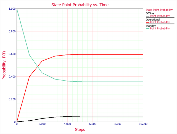
From the plot, we can also determine that the probabilities of being in a state reach steady-state after about 6 steps.
Continuous Markov Chains
A continuous Markov chain can be viewed as a Markov chain where the transitions between states are defined by (constant) transition rates, as opposed to transition probabilities at fixed steps. It is common to use continuous Markov chains when analyzing system reliability/availability problems.
Because we are no longer performing analysis using fixed probabilities and a fixed step, we are no longer able to simply multiply a state probability vector with a transition matrix in order to obtain new state probabilities after a given step.
Instead, our problem can be written as a system of ordinary differential equations, where each differential equation represents the change in the probability of being in a particular state:
- [math]\displaystyle{ \frac{dP_j}{dt}= \displaystyle\sum_{l=1}^{n} \lambda_{lj}P_{l} - \displaystyle\sum_{l=1}^{n} \lambda_{jl}P_{j}\,\! }[/math]
where:
- [math]\displaystyle{ n\,\! }[/math] is the total number of states
- [math]\displaystyle{ P_j\,\! }[/math] is the probability of being in state [math]\displaystyle{ j\,\! }[/math]
- [math]\displaystyle{ P_l\,\! }[/math] is the probability of being in state [math]\displaystyle{ l\,\! }[/math]
- [math]\displaystyle{ \lambda_{lj}\,\! }[/math] transition rate from state [math]\displaystyle{ l\,\! }[/math] to state [math]\displaystyle{ j\,\! }[/math]
- [math]\displaystyle{ \lambda_{jl}\,\! }[/math] transition rate from state [math]\displaystyle{ j\,\! }[/math] to state [math]\displaystyle{ l\,\! }[/math]
Our initial conditions to solve the differential equations are our initial probabilities for each state.
As a quick example, let us take a system that can be in one of two states, either working or under repair, and is initially in the working state. The transition rate from working to repair is 0.0001/hour (MTTF of 10,000 hours) and the transition rate from repair to working is 0.01/hour (MTTR of 100 hours). In this case, the two differential equations would look like this:
- [math]\displaystyle{ \frac{dP_{working}}{dt}=0.01\cdot P_{repair} - 0.0001 \cdot P_{working} \,\! }[/math]
- [math]\displaystyle{ \frac{dP_{repair}}{dt}=0.0001\cdot P_{working} - 0.01 \cdot P_{repair} \,\! }[/math]
with initial bounds of:
- [math]\displaystyle{ P_{working}(0)=1 \,\! }[/math]
- [math]\displaystyle{ P_{repair}(0)=0 \,\! }[/math]
Solving this system of equations yields the following results:
- [math]\displaystyle{ P_{working}=\frac{0.01}{0.0101}+\frac{0.0001}{0.0101}e^{-(0.0101)t} \,\! }[/math]
- [math]\displaystyle{ P_{repair}=\frac{0.0001}{0.0101}-\frac{0.0001}{0.0101}e^{-(0.0101)t} \,\! }[/math]
For more complex analyses, numerical methodologies are preferred. There are many methods, both analytical and numerical, to solve systems of ordinary differential equations. One of these is the Runge-Kutta-Fehlberg method, also known as the RKF45 method, which is a numerical algorithm. This algorithm is practical because one extra calculation allows for the error to be estimated and controlled with the use of an automatic adaptive step size methodology.
The methodology uses a 4th order Runge-Kutta and a 5th order Runge-Kutta, where the former is used for the calculation and the latter is used for the error estimation. The formulas for the method are as follows:
- [math]\displaystyle{ f_j=\frac{dP_{j}}{dt}= \displaystyle\sum_{l=1}^{n} \lambda_{lj}P_{l} - \displaystyle\sum_{l=1}^{n} \lambda_{jl}P_{j} \,\! }[/math]
- [math]\displaystyle{ k_1=hf(t_i,P_{l,i})\,\! }[/math]
- [math]\displaystyle{ k_2=hf\Big( t_i+\frac{h}{4},P_{l,i}+\frac{k_1}{4}\Big)\,\! }[/math]
- [math]\displaystyle{ k_3=hf\Big( t_i+\frac{3h}{8},P_{l,i}+\frac{3}{32}k_2\Big)\,\! }[/math]
- [math]\displaystyle{ k_4=hf\Big( t_i+\frac{12h}{13},P_{l,i}+\frac{1932}{2197}k_1+\frac{7200}{2197}k_2+\frac{7296}{2197}k_3\Big)\,\! }[/math]
- [math]\displaystyle{ k_5=hf\Big( t_i+h,P_{l,i}+\frac{439}{216}k_1+8k_2+\frac{3680}{513}k_3-\frac{845}{4104}k_4\Big)\,\! }[/math]
- [math]\displaystyle{ k_6=hf\Big( t_i+\frac{h}{2},P_{l,i}-\frac{8}{27}k_1+2k_2-\frac{3544}{2565}k_3+\frac{1859}{4104}k_4-\frac{11}{40}k_5\Big)\,\! }[/math]
- [math]\displaystyle{ P_{j,i+1}=P_{j,i}+\frac{25}{216}k_1+\frac{1408}{2565}k_3+\frac{2197}{4104}k_4-\frac{1}{5}k_5\,\! }[/math]
- [math]\displaystyle{ \tilde{P}_{j,i+1}=P_{j,i}+\frac{16}{135}k_1+\frac{6656}{12825}k_3+\frac{28561}{56430}k_4-\frac{9}{50}k_5+\frac{2}{55}k_6\,\! }[/math]
- [math]\displaystyle{ R=\frac{1}{h}|\tilde{P}_{j,i+1}-P_{j,i+1}|\,\! }[/math]
- [math]\displaystyle{ \delta=0.84\Big(\frac{\epsilon}{R}\Big)^{\frac{1}{4}}\,\! }[/math]
If [math]\displaystyle{ R\leq\epsilon\,\! }[/math] then keep [math]\displaystyle{ P_{i+1}\,\! }[/math] as the current solution, and move to next step with step size [math]\displaystyle{ \delta{h}\,\! }[/math]; if [math]\displaystyle{ R\gt \epsilon\,\! }[/math] then recalculate the current step with step size [math]\displaystyle{ \delta{h}\,\! }[/math]
where:
- [math]\displaystyle{ P_j\,\! }[/math] is the probability of being in state [math]\displaystyle{ j\,\! }[/math]
- [math]\displaystyle{ P_{l,i}\,\! }[/math] is the probability of being in state [math]\displaystyle{ l\,\! }[/math] at time [math]\displaystyle{ i\,\! }[/math]
- [math]\displaystyle{ \lambda_{lj}\,\! }[/math] is the transition rate from state [math]\displaystyle{ l\,\! }[/math] to state [math]\displaystyle{ j\,\! }[/math]
- [math]\displaystyle{ \lambda_{jl}\,\! }[/math] is the transition rate from state [math]\displaystyle{ j\,\! }[/math] to state [math]\displaystyle{ l\,\! }[/math]
- [math]\displaystyle{ f_j\,\! }[/math] is the change in the probability of being in state [math]\displaystyle{ P_j\,\! }[/math] (note that [math]\displaystyle{ f_j\,\! }[/math] is not a function of time for constant transition rate Markov chains)
- [math]\displaystyle{ h\,\! }[/math] is the time step size
- [math]\displaystyle{ t_i\,\! }[/math] is the time at [math]\displaystyle{ i\,\! }[/math]
- [math]\displaystyle{ \varepsilon\,\! }[/math] is the chosen acceptable error
This methodology can then be used for each state at each time step, where a time step is accepted only if the time step size is acceptable for each state in the system.
Since continuous Markov chains are often used for system availability/reliability analyses, the continuous Markov chain diagram in BlockSim allows the user the ability to designate one or more states as unavailable states. This allows for the calculation of both availability and reliability of the system.
Availability is calculated as the mean probability that the system is in a state that is not an unavailable state.
Reliability is calculated in the same manner as availability, with the additional restriction that all transitions leaving any unavailable state are considered to have a transition rate of zero.
Example
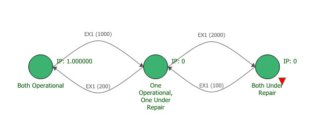
Assume you have a system composed of two generators. The system can be in one of three states:
- Both generators are operational
- One generator is operational and the other is under repair
- Both generators are under repair. This is an unavailable state.
The system starts in the state in which both generators are operational.
We know that the failure rate of a generator is 1 per 2,000 hours, and the repair rate is 1 per 200 hours.
Therefore:
- The transition rate from the state in which both generators are operational to the state where only one is operational is 1 per 1,000 hours.
- The transition rate from the state in which one generator is operational to the state where both generators are operational is 1 per 200 hours.
- The transition rate from the state in which one generator is operational to the state where both generators are under repair is 1 per 2,000 hours.
- The transition rate from the state in which both generators are under repair to the state where one generator is operational is 1 per 100 hours.
We would like to know the mean availability of our system after 20,000 hours for all three states so that we can estimate our output based on time spent at full, half and zero generator capacity.
Solving this system by hand using the RKF45 method would be very time consuming, so we will turn to BlockSim to help us solve this problem using a continuous Markov diagram. After creating the diagram, adding the states and the transition rates, the final diagram looks like this:
Once the diagram is complete, the analysis is set for 20,000 hours. The comparison between the mean probabilities of the states can be done using a bar graph, or by looking at the diagram result summary.
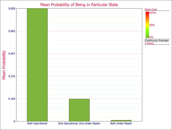
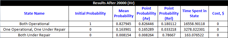
From the Mean Probability column, we can see that the system is expected to be fully operational 82.8% of the time, half operational 16.4% of the time, and non-operational 0.8% of the time.
From the Point Probability (Av) column, we can get the point probability of being in a state when all transitions are considered. From the Point Probability (Rel) column, we can get the point probability of being in a state if we assume that there is no return from unavailable states, or in other words we are assuming no repair once the system has entered an unavailable (failed) state. Using the "non-repair" assumption, there is only an 18.0% chance that the system would still be fully operational, a 3.3% chance that it would be half operational and a 78.7% chance that it would be non-operational.
Phases
It is possible to do analyses with multiple phases for both discrete and continuous Markov chain calculations. When using phases, the software keeps track of state correspondence across phases using the name of the state (e.g., "State B" is one phase is considered to correspond to "State B" in all other phases). The starting state probability comes from the ending state probability from the previous phase. If a state is absent from a phase, then its state probability does not change during the phase.
Also, it is possible to perform an analysis where the number of steps, for discrete analyses, or the operational time, for continuous analyses, are greater/longer than the sum length of all the phases. In this case, the analysis will return to the first phase, without resetting the state probabilities, and continue from there.