Mixture Design

Introduction
When a product is formed by mixing together two or more ingredients, the product is called a mixture, and the ingredients are called mixture components. In a general mixture problem, the measured response is assumed to depend only on the proportions of the ingredients in the mixture, not the amount of the mixture. For example, the taste of a fruit punch recipe (i.e., the response) might depend on the proportions of watermelon, pineapple and orange juice in the mixture. The taste of a small cup of fruit punch will obviously be the same as a big cup.
Sometimes the responses of a mixture experiment depend not only on the proportions of ingredients, but also on the settings of variables in the process of making the mixture. For example, the tensile strength of stainless steel is not only affected by the proportions of iron, copper, nickel and chromium in the alloy; it is also affected by process variables such as temperature, pressure and curing time used in the experiment.
One of the purposes of conducting a mixture experiment is to find the best proportion of each component and the best value of each process variable, in order to optimize a single response or multiple responses simultaneously. In this chapter, we will discuss how to design effective mixture designs and how to analyze data from mixture experiments with and without process variables.
Mixture Design Types
There are several different types of mixture designs. The most common ones are simplex lattice, simplex centroid, simplex axial and extreme vertex designs, each of which is used for a different purpose.
- If there are many components in a mixture, the first choice is to screen out the most important ones. Simplex axial and Simplex centroid designs are used for this purpose.
- If the number of components is not large, but a high order polynomial equation is needed in order to accurately describe the response surface, then a simplex lattice design can be used.
- Extreme vertex designs are used for the cases when there are constraints on one or more components (e.g., if the proportion of watermelon juice in a fruit punch recipe is required to be less than 30%, and the combined proportion of watermelon and orange juice should always be between 40% and 70%).
Simplex Plot
Since the sum of all the mixture components is always 100%, the experiment space usually is given by a plot. The experiment space for the fruit punch experiment is given in the following triangle or simplex plot.
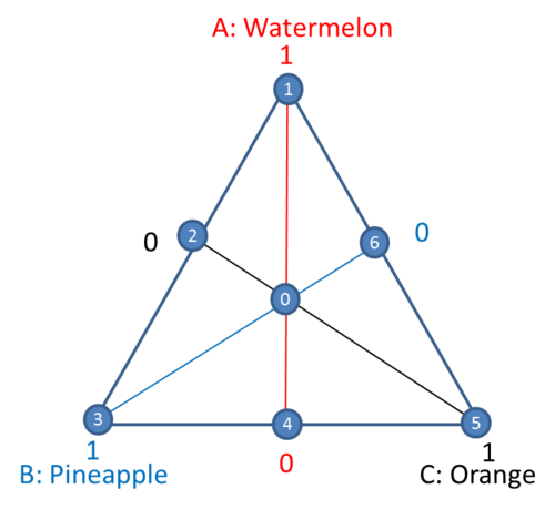
The triangle area in the above plot is defined by the fact that the sum of the three ingredients is 1 (100%). For the points that are on the vertices, the punch only has one ingredient. For instance, point 1 only has watermelon. The line opposite of point 1 represents a mixture with no watermelon .
The coordinate system used for the value of each ingredient [math]\displaystyle{ {{x}_{i}}\,\! }[/math],[math]\displaystyle{ i=1,2,...,q\,\! }[/math] is called a simplex coordinate system. q is the number of ingredients. The simplex plot can only visually display three ingredients. If there are more than three ingredients, the values for other ingredients must be provided. For the fruit punch example, the coordinate for point 1 is (1, 0, 0). The interior points of the triangle represent mixtures in which none of the three components is absent. It means all [math]\displaystyle{ {{x}_{i}}\gt 0\,\! }[/math], [math]\displaystyle{ i=1,2,3\,\! }[/math]. Point 0 in the middle of the triangle is called the center point. In this case, it is the centroid of a face/plane. The coordinate for point 0 is (1/3, 1/3, 1/3). Points 2, 4 and 6 are each called a centroid of edge. Their coordinates are (0.5, 0.5, 0), (0, 0.5, 0.5), and (0.5, 0, 0.5).
Simplex Lattice Design
The response in a mixture experiment usually is described by a polynomial function. This function represents how the components affect the response. To better study the shape of the response surface, the natural choice for a design would be the one whose points are spread evenly over the whole simplex. An ordered arrangement consisting of a uniformly spaced distribution of points on a simplex is known as a lattice.
A {q, m} simplex lattice design for q components consists of points defined by the following coordinate settings: the proportions assumed by each component take the m+1 equally spaced values from 0 to 1,
- [math]\displaystyle{ {{x}_{i}}=0,\frac{1}{m},\frac{2}{m},....,1\text{ }i=1,2,....,q\,\! }[/math]
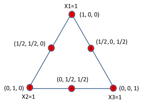
and the design space consists of all the reasonable combinations of all the values for each factor. m is usually called the degree of the lattice. For example, for a {3, 2} design, [math]\displaystyle{ {{x}_{i}}=0,\frac{1}{2},1\,\! }[/math] and its design space has 6 points. They are:
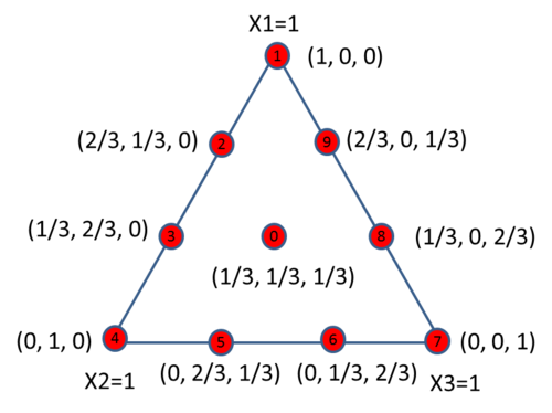
For a {3, 3} design, [math]\displaystyle{ {{x}_{i}}=0,\frac{1}{3},\frac{2}{3},1\,\! }[/math], and its design space has 10 points. They are:
For a simplex design with degree of m, each component has m + 1 different values, therefore, the experiment results can be used to fit a polynomial equation up to an order of m. A {3, 3} simplex lattice design can be used to fit the following model.
- [math]\displaystyle{ \begin{align} & y={{\beta }_{1}}{{x}_{1}}+{{\beta }_{2}}{{x}_{2}}+{{\beta }_{3}}{{x}_{3}}+{{\beta }_{12}}{{x}_{1}}{{x}_{2}}+{{\beta }_{13}}{{x}_{1}}{{x}_{3}}+{{\beta }_{23}}{{x}_{2}}{{x}_{3}} \\ & +{{\delta }_{12}}{{x}_{1}}{{x}_{2}}\left( {{x}_{1}}-{{x}_{2}} \right)+{{\delta }_{13}}{{x}_{1}}{{x}_{3}}\left( {{x}_{1}}-{{x}_{3}} \right)+{{\delta }_{23}}{{x}_{2}}{{x}_{3}}\left( {{x}_{2}}-{{x}_{3}} \right) \\ & +{{\beta }_{123}}{{x}_{1}}{{x}_{2}}{{x}_{3}} \end{align}\,\! }[/math]
The above model is called the full cubic model. Note that the intercept term is not included in the model due to the correlation between all the components (their sum is 100%).
Simplex lattice design includes all the component combinations. For a {q, m} design, the total number of runs is [math]\displaystyle{ \left( \begin{align} & q+m-1 \\ & m \\ \end{align} \right)\,\! }[/math]. Therefore to reduce the number of runs and still be able to fit a high order polynomial model, sometimes we can use simplex centroid design which is explained next.
Simplex Centroid Design
A simplex centroid design only includes the centroid points. For the components that appear in a run in a simplex centroid design, they have the same values.
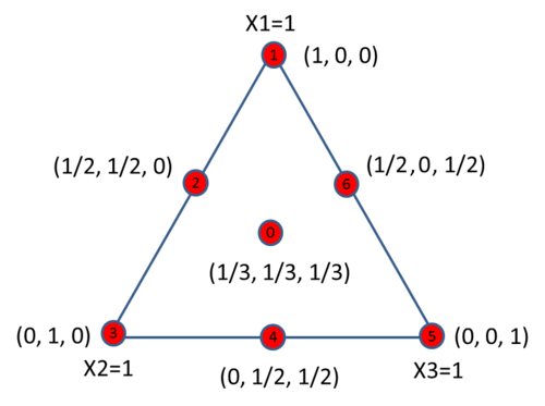
In the above simplex plot, points 2, 4 and 6 are 2nd degree centroids. Each of them has two non-zero components with equal values. Point 0 is a 3rd degree centroid and all three components have the same value. For a design with q components, the highest degree of centroid is q. It is called the overall centroid, or the center point of the design.
For a q component simplex centroid design with a degree of centroid of q, the total number of runs is [math]\displaystyle{ {{2}^{q}}-1\,\! }[/math]. The runs correspond to the q permutations of (1, 0, 0,…, 0), [math]\displaystyle{ \left( \begin{align} & q \\ & 2 \\ \end{align} \right)\,\! }[/math] permutations of (1/2, 1/2, 0, 0, 0, 0, …,0), the [math]\displaystyle{ \left( \begin{align} & q \\ & 3 \\ \end{align} \right)\,\! }[/math] permutations of (1/3, 1/3, 1/3, 0, 0, 0, 0,…, 0)…., and the overall centroid (1/q, 1/q, …, 1/q). If the degree of centroid is defined as [math]\displaystyle{ m\,\! }[/math] (m < q), then the total number of runs will be [math]\displaystyle{ \left( \begin{align} & q \\ & 1 \\ \end{align} \right)+\left( \begin{align} & q \\ & 2 \\ \end{align} \right)+...+\left( \begin{align} & q \\ & m \\ \end{align} \right)\,\! }[/math].
Since a simplex centroid design usually has fewer runs than a simplex lattice design with the same degree, a polynomial model with fewer terms should be used. A {3, 3} simplex centroid design can be used to fit the following model.
- [math]\displaystyle{ y={{\beta }_{1}}{{x}_{1}}+{{\beta }_{2}}{{x}_{2}}+{{\beta }_{3}}{{x}_{3}}+{{\beta }_{12}}{{x}_{1}}{{x}_{2}}+{{\beta }_{13}}{{x}_{1}}{{x}_{3}}+{{\beta }_{23}}{{x}_{2}}{{x}_{3}}+{{\beta }_{123}}{{x}_{1}}{{x}_{2}}{{x}_{3}}\,\! }[/math]
The above model is called the special cubic model. Note that the intercept term is not included due to the correlation between all the components (their sum is 100%).
Simplex Axial Design
The simplex lattice and simplex centroid designs are boundary designs since the points of these designs are positioned on boundaries (vertices, edges, faces, etc.) of the simplex factor space, with the exception of the overall centroid. Axial designs, on the other hand, are designs consisting mainly of the points positioned inside the simplex. Axial designs have been recommended for use when component effects are to be measured in a screening experiment, particularly when first degree models are to be fitted.
Definition of Axial: The axial of a component [math]\displaystyle{ i\,\! }[/math] is defined as the imaginary line extending from the base point [math]\displaystyle{ {{x}_{i}}=0\,\! }[/math], [math]\displaystyle{ {{x}_{j}}=1/\left( q-1 \right)\,\! }[/math] for all [math]\displaystyle{ j\ne i\,\! }[/math], to the vertex where [math]\displaystyle{ {{x}_{i}}=1,{{x}_{j}}=0\,\! }[/math] all [math]\displaystyle{ j\ne i\,\! }[/math]. [John Cornell]
In a simplex axial design, all the points are on the axial. The simplest form of axial design is one whose points are positioned equidistant from the overall centroid [math]\displaystyle{ \left( {1}/{q,{1}/{q,}\;{1}/{q,}\;...}\; \right)\,\! }[/math]. Traditionally, points located at the half distance from the overall centroid to the vertex are called axial points/blends. This is illustrated in the following plot.
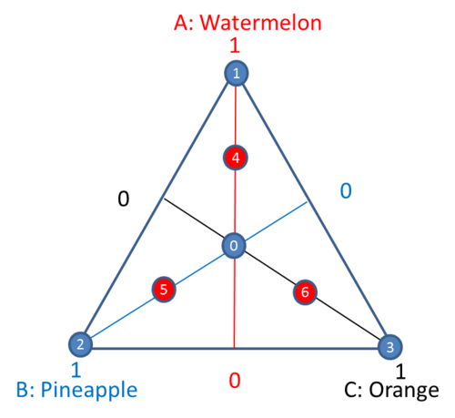
Points 4, 5 and 6 are the axial blends.
By default, a simple axial design in a DOE folio only has vertices, axial blends, centroid of the constraint planes and the overall centroid. For a design with q components, constraint plane centroids are the center points of dimension of q-1 space. One component is 0, and the remaining components have the same values for the center points of constraint planes. The number of the constraint plane centroids is the number of components q. The total number of runs in a simple axial design will be 3q+1. They are q vertex runs, q centroids of constraint planes, q axial blends and 1 overall centroid.
A simplex axial design for 3 components has 10 points as given below.
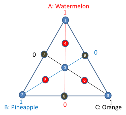
Points 1, 2 and 3 are the three vertices; points 4, 5, 6 are the axial blends; points 7, 8 and 9 are the centroids of constraint planes, and point 0 is the overall center point.
Extreme Vertex Design
Extreme vertex designs are used when both lower and upper bound constraints on the components are presented, or when linear constraints are added to several components. For example, if a mixture design with 3 components has the following constraints:
- [math]\displaystyle{ {{x}_{2}}\le 0.7\,\! }[/math]
- [math]\displaystyle{ -2{{x}_{1}}+2{{x}_{2}}+3{{x}_{3}}\ge 0\,\! }[/math]
- [math]\displaystyle{ 48{{x}_{1}}+13{{x}_{2}}-{{x}_{3}}\ge 0\,\! }[/math]
Then the feasible region is defined by the six points in the following simplex plot. To meet the above constraints, all the runs conducted in the experiment should be in the feasible region or on its boundary.
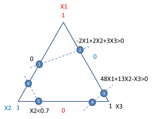
The CONSIM method described in [Snee 1979] is used in a Weibull++ DOE folio to check the consistency of all the constraints and to get the vertices defined by them.
Extreme vertex designs by default use the vertices at the boundary. Additional points such as the centroid of spaces of different dimensions, axial points and the overall center point can be added. In extreme vertex designs, axial points are between the overall center point and the vertices. For the above example, if the axial points and the overall center point are added, then all the runs in the experiment will be:
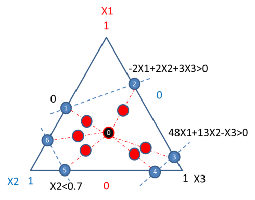
Point 0 in the center of the feasible region is the overall centroid. The other red points are the axial points. They are at the middle of the lines connecting the center point with the vertices.
Mixture Design Data Analysis
In the following section, we will discuss the most popular regression models in mixture design data analysis. Due to the correlation between all the components in mixture designs, the intercept term usually is not included in the regression model.
Models Used in Mixture Design
For a design with three components, the following models are commonly used.
- Linear model:
- [math]\displaystyle{ y={{\beta }_{1}}{{x}_{1}}+{{\beta }_{2}}{{x}_{2}}+{{\beta }_{3}}{{x}_{3}}\,\! }[/math]
If the intercept were included in the model, then the linear model would be
- [math]\displaystyle{ y=\beta _{0}^{'}+\beta _{1}^{'}{{x}_{1}}+\beta _{2}^{'}{{x}_{2}}+\beta _{3}^{'}{{x}_{3}}\,\! }[/math]
However, since [math]\displaystyle{ {{x}_{1}}+{{x}_{2}}+{{x}_{3}}=1\,\! }[/math] (can be other constants as well), the above equation can be written as
- [math]\displaystyle{ \begin{align} & y=\beta _{0}^{'}\left( {{x}_{1}}+{{x}_{2}}+{{x}_{3}} \right)+\beta _{1}^{'}{{x}_{1}}+\beta _{2}^{'}{{x}_{2}}+\beta _{3}^{'}{{x}_{3}} \\ & =\left( \beta _{0}^{'}+\beta _{1}^{'} \right){{x}_{1}}+\left( \beta _{0}^{'}+\beta _{2}^{'} \right){{x}_{2}}+\left( \beta _{0}^{'}+\beta _{3}^{'} \right){{x}_{3}} \\ & ={{\beta }_{1}}{{x}_{1}}+{{\beta }_{2}}{{x}_{2}}+{{\beta }_{3}}{{x}_{3}} \end{align}\,\! }[/math]
The equation has thus been reformatted to omit the intercept.
- Quadratic model:
- [math]\displaystyle{ y={{\beta }_{1}}{{x}_{1}}+{{\beta }_{2}}{{x}_{2}}+{{\beta }_{3}}{{x}_{3}}+{{\beta }_{12}}{{x}_{1}}{{x}_{2}}+{{\beta }_{13}}{{x}_{1}}{{x}_{3}}+{{\beta }_{23}}{{x}_{2}}{{x}_{3}}\,\! }[/math]
There are no classic quadratic terms such as [math]\displaystyle{ x_{1}^{2}\,\! }[/math]. This is because
- [math]\displaystyle{ x_{1}^{2}={{x}_{1}}\left( 1-{{x}_{2}}-{{x}_{3}} \right)={{x}_{1}}-{{x}_{1}}{{x}_{2}}-{{x}_{1}}{{x}_{3}}\,\! }[/math]
- Full cubic model:
- [math]\displaystyle{ \begin{align} & y={{\beta }_{1}}{{x}_{1}}+{{\beta }_{2}}{{x}_{2}}+{{\beta }_{3}}{{x}_{3}}+{{\beta }_{12}}{{x}_{1}}{{x}_{2}}+{{\beta }_{13}}{{x}_{1}}{{x}_{3}}+{{\beta }_{23}}{{x}_{2}}{{x}_{3}} \\ & +{{\delta }_{12}}{{x}_{1}}{{x}_{2}}\left( {{x}_{1}}-{{x}_{2}} \right)+{{\delta }_{13}}{{x}_{1}}{{x}_{3}}\left( {{x}_{1}}-{{x}_{3}} \right)+{{\delta }_{23}}{{x}_{2}}{{x}_{3}}\left( {{x}_{2}}-{{x}_{3}} \right) \\ & +{{\beta }_{123}}{{x}_{1}}{{x}_{2}}{{x}_{3}} \end{align}\,\! }[/math]
- Special cubic model: [math]\displaystyle{ {{\delta }_{ij}}{{x}_{i}}{{x}_{j}}\left( {{x}_{i}}-{{x}_{j}} \right)\,\! }[/math] are removed from the full cubic model.
- [math]\displaystyle{ \begin{align} & y={{\beta }_{1}}{{x}_{1}}+{{\beta }_{2}}{{x}_{2}}+{{\beta }_{3}}{{x}_{3}}+{{\beta }_{12}}{{x}_{1}}{{x}_{2}}+{{\beta }_{13}}{{x}_{1}}{{x}_{3}}+{{\beta }_{23}}{{x}_{2}}{{x}_{3}} \\ & +{{\beta }_{123}}{{x}_{1}}{{x}_{2}}{{x}_{3}} \end{align}\,\! }[/math]
The above types of models are called Scheffe type models. They can be extended to designs with more than three components.
In regular regression analysis, the effect of an exploratory variable or factor is represented by the value of the coefficient. The ratio of the estimated coefficient and its standard error is used for the t-test. The t-test can tell us if a coefficient is 0 or not. If a coefficient is statistically 0, then the corresponding factor has no significant effect on the response. However, for Scheffe type models, since the intercept term is not included in the model, we cannot use the regular t-test to test each individual main effect. In other words, we cannot test if the coefficient for each component is 0 or not.
Similarly, in the ANOVA analysis, the linear effects of all the components are tested together as a single group. The main effect test for each individual component is not conducted. To perform ANOVA analysis, the Scheffe type model needs to be reformatted to include the hidden intercept. For example, the linear model
- [math]\displaystyle{ y={{\beta }_{1}}{{x}_{1}}+{{\beta }_{2}}{{x}_{2}}+{{\beta }_{3}}{{x}_{3}}\,\! }[/math]
can be rewritten as
- [math]\displaystyle{ \begin{align} & y={{\beta }_{1}}{{x}_{1}}+{{\beta }_{2}}{{x}_{2}}+{{\beta }_{3}}{{x}_{3}} \\ & ={{\beta }_{1}}{{x}_{1}}+{{\beta }_{2}}{{x}_{2}}+{{\beta }_{3}}\left( 1-{{x}_{1}}-{{x}_{2}} \right) \\ & ={{\beta }_{3}}+\left( {{\beta }_{1}}-{{\beta }_{3}} \right){{x}_{1}}+\left( {{\beta }_{2}}-{{\beta }_{3}} \right){{x}_{2}} \\ & ={{\beta }_{0}}+\beta _{1}^{'}{{x}_{1}}+\beta _{2}^{'}{{x}_{2}} \end{align}\,\! }[/math]
where [math]\displaystyle{ {{\beta }_{0}}={{\beta }_{3}}\,\! }[/math], [math]\displaystyle{ \beta _{1}^{'}={{\beta }_{1}}-{{\beta }_{3}}\,\! }[/math], [math]\displaystyle{ \beta _{2}^{'}={{\beta }_{2}}-{{\beta }_{3}}\,\! }[/math]. All other models such as the quadratic, cubic and special cubic model can be reformatted using the same procedure. By including the intercept in the model, the correct sum of squares can be calculated in the ANOVA table. If ANOVA analysis is conducted directly using the Scheffe type models, the result will be incorrect.
L-Pseudocomponent, Proportion, and Actual Values
In mixture designs, the total amount of the mixture is usually given. For example, we can make either a one-pound or a two-pound cake. Regardless of whether the cake is one or two pounds, the proportion of each ingredient is the same. When the total amount is given, the upper and lower limits for each ingredient are usually given in amounts, which is easier for the experimenter to understand. Of course, if the limits or other constraints are given in terms of proportions, these proportions need be converted to the real amount values when conducting the experiment. To keep everything consistent, all the constraints in a DOE folio are treated as amounts.
In regular factorial design and response surface methods, the regression model is calculated using coded values. Coded values scale all the factors to the same magnitude, which makes the analysis much easier and reduces convergence error. Similarly, the analysis in mixture design is conducted using the so-called L-pseudocomponent value. L-pseudocomponent values scale all the components' values within 0 and 1. In a DOE folio all the designs and calculations for mixture factors are based on L-pseudocomponent values. The relationship between L-pseudocomponent values, proportions and actual amounts are explained next.
Example for L-Pseudocomponent Value
We are going to make one gallon (about 3.8 liters) of fruit punch. Three ingredients will be in the punch with the following constraints.
- [math]\displaystyle{ 1.2\le A\le 3.8\,\! }[/math], [math]\displaystyle{ 1.5\le B\le 3\,\! }[/math], [math]\displaystyle{ 0\le C\le 3.8\,\! }[/math]
Let [math]\displaystyle{ x_{i}^{A}\,\! }[/math] (i = 1, 2, 3) be the actual amount value, [math]\displaystyle{ x_{i}^{{}}\,\! }[/math] be the L-pseudocomponent value and [math]\displaystyle{ x_{i}^{R}\,\! }[/math] be the proportion value. Then the equations for the conversion between them are:
- [math]\displaystyle{ {{x}_{i}}=\frac{x_{i}^{A}-{{l}_{i}}}{\left( T-\sum\limits_{j=1}^{p}{{{l}_{j}}} \right)}\,\! }[/math], [math]\displaystyle{ x_{i}^{A}={{l}_{i}}+\left( T-\sum\limits_{j=1}^{p}{{{l}_{i}}} \right){{x}_{i}}\,\! }[/math], [math]\displaystyle{ x_{i}^{R}=\frac{x_{i}^{A}}{T}\,\! }[/math]
where [math]\displaystyle{ {{x}_{1}}\,\! }[/math], [math]\displaystyle{ x_{1}^{A}\,\! }[/math] and
[math]\displaystyle{ x_{1}^{R}\,\! }[/math] are for component A, [math]\displaystyle{ {{x}_{2}}\,\! }[/math], [math]\displaystyle{ x_{2}^{A}\,\! }[/math] and [math]\displaystyle{ x_{2}^{R}\,\! }[/math] are for component B, and [math]\displaystyle{ {{x}_{3}}\,\! }[/math], [math]\displaystyle{ x_{3}^{A}\,\! }[/math] and [math]\displaystyle{ x_{3}^{R}\,\! }[/math] are for component C.
Since components in this example have both lower and upper limit constraints, an extreme vertex design is used. The design settings are given below.

The created design in terms of L-pseudocomponent values is:

Displayed in amount values, it is:

Displayed in proportion values, it is:

Check Constraint Consistency
In the above example, all the constraints are consistent. However, if we set the constraints to
- [math]\displaystyle{ 1.2\le A\le 3.8\,\! }[/math], [math]\displaystyle{ 1.5\le B\le 3\,\! }[/math], [math]\displaystyle{ 2\le C\le 3.8,\,\! }[/math]
then they are not consistent. This is because the total is only 3.8, but the sum of all the lower limits is 4.7. Therefore, not all the lower limits can be satisfied at the same time. If only lower limits and upper limits are presented for all the components, then we can adjust the lower bounds to make the constraints consistent. The method given by [Pieple 1983] is used and summarized below.
Defined the range of a component to be [math]\displaystyle{ {{R}_{i}}={{U}_{i}}-{{L}_{i}}\,\! }[/math]. [math]\displaystyle{ {{U}_{i}}\,\! }[/math] and [math]\displaystyle{ {{L}_{i}}\,\! }[/math] are the upper and lower limit for component i. The implied range of component i is [math]\displaystyle{ R_{i}^{*}=U_{i}^{*}-L_{i}^{*}\,\! }[/math], where [math]\displaystyle{ L_{i}^{*}=T-\sum\limits_{j\ne i}^{q}{{{U}_{i}}}\,\! }[/math], and [math]\displaystyle{ U_{i}^{*}=T-\sum\limits_{j\ne i}^{q}{{{L}_{i}}}\,\! }[/math]. T is the total amount. The steps for checking and adjusting bounds are given below.
Step 1: Check if [math]\displaystyle{ L_{i}^{*}\,\! }[/math] and [math]\displaystyle{ U_{i}^{*}\,\! }[/math] are greater than 0, if they are, then these constraints meet the basic requirement to be consistent. We can move forward to step 2. If not, these constraints cannot be adjusted to be consistent. We should stop.
Step 2: For each component, check if [math]\displaystyle{ {{L}_{i}}\ge L_{i}^{*}\,\! }[/math] and [math]\displaystyle{ {{U}_{i}}\le U_{i}^{*}\,\! }[/math]. If they are, then this component’s constraints are consistent. Otherwise, if [math]\displaystyle{ {{L}_{i}}\lt L_{i}^{*}\,\! }[/math], then set [math]\displaystyle{ {{L}_{i}}=L_{i}^{*}\,\! }[/math], and if [math]\displaystyle{ {{U}_{i}}\gt U_{i}^{*}\,\! }[/math], then set [math]\displaystyle{ {{U}_{i}}=U_{i}^{*}\,\! }[/math].
Step 3: Whenever a bound is changed, restart from Step 1 to use the new bound to check if all the constraints are consistent. Repeat this until all the limits are consistent.
For extreme vertex design where linear constraints are allowed, the DOE folio will give a warning and stop creating the design if inconsistent linear combination constraints are found. No adjustment will be conducted for linear constraints.
Response Trace Plot
Due to the correlation between all the components, the regular t-test is not used to test the significance of each component. A special plot called the Response Trace Plot can be used to see how the response changes when each component changes from its reference point [John Cornell].
A reference point can be any point inside the experiment space. An imaginary line can be drawn from this reference point to each vertex [math]\displaystyle{ {{x}_{i}}=1\,\! }[/math], and [math]\displaystyle{ {{x}_{j}}=0\,\! }[/math] ([math]\displaystyle{ i\ne j\,\! }[/math]). This line is the direction for component i to change. Component i can either increase or decrease its value along this line, while the ratio of other components [math]\displaystyle{ {{{x}_{j}}}/{{{x}_{k}}}\,\! }[/math] ([math]\displaystyle{ j,k\ne i\,\! }[/math]) will keep constant. If the simplex plot is defined in terms of proportion, then the direction is called Cox’s direction, and [math]\displaystyle{ {{{x}_{j}}}/{{{x}_{k}}}\,\! }[/math] is the ratio of proportion. If the simplex plot is defined in terms of pseduocomponent value, then the direction is called Pieple’s direction, and [math]\displaystyle{ {{{x}_{j}}}/{{{x}_{k}}}\,\! }[/math] will be the ratio of pseduocomponent values.
Assume the reference point in terms of proportion is [math]\displaystyle{ s=\left( {{s}_{1}},{{s}_{2}},...,{{s}_{q}} \right)\,\! }[/math] where [math]\displaystyle{ {{s}_{1}}+{{s}_{2}}+...+{{s}_{q}}=1\,\! }[/math]. Suppose the proportion of component [math]\displaystyle{ i\,\! }[/math] at [math]\displaystyle{ {{s}_{i}}\,\! }[/math] is now changed by [math]\displaystyle{ {{\Delta }_{i}}\,\! }[/math] ([math]\displaystyle{ {{\Delta }_{i}}\,\! }[/math] could be greater than or less than 0) in Cox’s direction, so that the new proportion becomes [math]\displaystyle{ {{x}_{i}}={{s}_{i}}+{{\Delta }_{i}}\,\! }[/math]
Then the proportions of the remaining [math]\displaystyle{ q-1\,\! }[/math] components resulting from the change from [math]\displaystyle{ {{s}_{i}}\,\! }[/math] will be
- [math]\displaystyle{ {{x}_{j}}={{s}_{j}}-\frac{{{\Delta }_{i}}{{s}_{j}}}{1-{{s}_{i}}}\,\! }[/math]
After the change, the ratio of component j and k is unchanged. This is because
- [math]\displaystyle{ \frac{{{x}_{j}}}{{{x}_{k}}}=\frac{{{s}_{j}}-\frac{{{\Delta }_{i}}{{s}_{j}}}{1-{{s}_{i}}}}{{{s}_{k}}-\frac{{{\Delta }_{i}}{{s}_{k}}}{1-{{s}_{i}}}}=\frac{{{s}_{j}}}{{{s}_{k}}}\frac{\frac{{{\Delta }_{i}}}{1-{{s}_{i}}}}{\frac{{{\Delta }_{i}}}{1-{{s}_{i}}}}=\frac{{{s}_{j}}}{{{s}_{k}}}\,\! }[/math]
While [math]\displaystyle{ {{x}_{i}}\,\! }[/math] is changed along Cox’s direction, we can use a fitted regression model to get the response value y. A response trace plot for a mixture design with three components will look like

The x-axis is the deviation amount from the reference point, and the y-value is the fitted response. Each component has one curve. Since the red curve for component A changes significantly, this means it has a significant effect along its axial. The blue curve for component C is almost flat; this means when C changes along Cox’s direction and other components keep the same ratio, the response Y does not change very much. The effect of component B is between component A and C.
Example
Watermelon (A), pineapple (B) and orange juice (C) are used for making 3.8 liters of fruit punch. At least 30% of the fruit punch must be watermelon. Therefore the constraints are
- [math]\displaystyle{ 1.14\le A\le 3.8\,\! }[/math], [math]\displaystyle{ 0\le B\le 3.8\,\! }[/math], [math]\displaystyle{ 0\le C\le 3.8,\,\! }[/math]
Different blends of the three-juice recipe were evaluated by a panel. A value from 1 (extremely poor) to 9 (very good) is used for the response [John Cornell, page 74]. A {3, 2} simplex lattice design is used with one center point and three axial points. Three replicates were conducted for each ingredient combination. The settings for creating this design in a DOE folio is

The generated design in L-pseudocomponent values and the response values from the experiment are

The simplex design point plot is

Main effect and 2-way interactions are included in the regression model. The result for the regression model in terms of L-pseudocomponents is
- [math]\displaystyle{ y=4.81{{x}_{1}}+6.03{{x}_{2}}+6.16{{x}_{3}}+1.13{{x}_{1}}{{x}_{2}}+2.45{{x}_{1}}{{x}_{3}}+1.69{{x}_{2}}{{x}_{3}}\,\! }[/math]
The regression information table is
| Regression Information | |||||||
|---|---|---|---|---|---|---|---|
| Term | Coefficient | Standard Error | Low Confidence | High Confidence | T Value | P Value | Variance Inflation Factor |
| A: Watermelon | 4.8093 | 0.3067 | 4.2845 | 5.3340 | 1.9636 | ||
| B: Pineapple | 6.0274 | 0.3067 | 5.5027 | 6.5522 | 1.9636 | ||
| C: Orange | 6.1577 | 0.3067 | 5.6330 | 6.6825 | 1.9636 | ||
| A • B | 1.1253 | 1.4137 | -1.2934 | 3.5439 | 0.7960 | 0.4339 | 1.9819 |
| A • C | 2.4525 | 1.4137 | 0.0339 | 4.8712 | 1.7348 | 0.0956 | 1.9819 |
| B • C | 1.6889 | 1.4137 | -0.7298 | 4.1075 | 1.1947 | 0.2439 | 1.9819 |
The result shows that the taste of the fruit punch is significantly affected by the interaction between watermelon and orange.
The ANOVA table is
| Anova Table | |||||
|---|---|---|---|---|---|
| Source of Variation | Degrees of Freedom | Standard ErrorSum of Squares [Partial] | Mean Squares [Partial] | F Ratio | P Value |
| Model | 5 | 6.5517 | 1.3103 | 4.3181 | 0.0061 |
| Linear | 2 | 3.6513 | 1.8256 | 6.0162 | 0.0076 |
| A • B | 1 | 0.1923 | 0.1923 | 0.6336 | 0.4339 |
| A • C | 1 | 0.9133 | 0.9133 | 3.0097 | 0.0956 |
| B • C | 1 | 0.4331 | 0.4331 | 1.4272 | 0.2439 |
| Residual | 24 | 7.2829 | 0.3035 | ||
| Lack of Fit | 4 | 4.4563 | 1.1141 | 7.8825 | 0.0006 |
| Pure Error | 20 | 2.8267 | 0.1413 | ||
| Total | 29 | 13.8347 | |||
The simplex contour plot in L-pseudocomponent values is

From this plot we can see that as the amount of watermelon is reduced, the taste of the fruit punch becomes better.
In order to find the best proportion of each ingredient, the optimization tool in the Weibull++ DOE folio can be utilized. Set the settings as

The resulting optimal plot is

This plot shows that when the amounts for watermelon, pineapple and orange juice are 1.141, 1.299 and 1.359, respectively, the rated taste of the fruit punch is highest.
Mixture Design with Process Variables
Process variables often play very important roles in mixture experiments. A simple example is baking a cake. Even with the same ingredients, different baking temperatures and baking times can produce completely different results. In order to study the effect of process variables and find their best settings, we need to consider them when conducting a mixture experiment.
An easy way to do this is to make mixtures with the same ingredients in different combinations of process variables. If all the process variables are independent, then we can plan a regular factorial design for these process variables. By combining these designs with a separated mixture design, the effect of mixture components and effect of process variables can be studied.
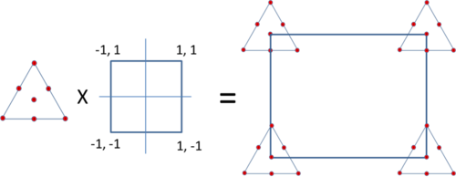
For example, a {3, 2} simplex lattice design is used for a mixture with 3 components. Together with the center point, it has total of 7 runs or 7 different ingredient combinations. Assume 2 process variables are potentially important and a two level factorial design is used for them. It has a total of 4 combinations for these 2 process variables. If the 7 different mixtures are made under each of the 4 process variable combinations, then the experiment has a total of 28 runs. This is illustrated in the figure below.
Of course, if it is possible, all the 28 experiments should be conducted in a random order.
Model with Process Variables
In a DOE folio, regression models including both mixture components and process variables are available. For mixture components, we use L-pseudocomponent values, and for process variables coded values are used.
Assume a design has 3 mixture components and 2 process variables, as illustrated in the above figure. We can use the following models for them.
- For the 3 mixture components, the following special cubic model is used.
- [math]\displaystyle{ y={{\beta }_{1}}{{x}_{1}}+{{\beta }_{2}}{{x}_{2}}+{{\beta }_{3}}{{x}_{3}}+{{\beta }_{12}}{{x}_{1}}{{x}_{2}}+{{\beta }_{13}}{{x}_{1}}{{x}_{3}}+{{\beta }_{23}}{{x}_{2}}{{x}_{3}}+{{\beta }_{123}}{{x}_{1}}{{x}_{2}}{{x}_{3}}\,\! }[/math]
- For the 2 process variables the following model is used.
- [math]\displaystyle{ y={{\alpha }_{0}}+{{\alpha }_{1}}{{z}_{1}}+{{\alpha }_{2}}{{z}_{2}}+{{\alpha }_{12}}{{z}_{1}}{{z}_{2}}\,\! }[/math]
- The combined model with both mixture components and process variables is
- [math]\displaystyle{ \begin{align} & y=\sum\limits_{i=1}^{3}{\gamma _{i}^{0}{{x}_{i}}}+\sum{\sum\limits_{i\lt j}^{3}{\gamma _{ij}^{0}{{x}_{i}}{{x}_{j}}}+}\gamma _{123}^{0}{{x}_{1}}{{x}_{2}}{{x}_{3}} \\ & +\left( \sum\limits_{i=1}^{3}{\gamma _{i}^{1}{{x}_{i}}}+\sum{\sum\limits_{i\lt j}^{3}{\gamma _{ij}^{1}{{x}_{i}}{{x}_{j}}}+}\gamma _{123}^{1}{{x}_{1}}{{x}_{2}}{{x}_{3}} \right){{z}_{1}} \\ & +\left( \sum\limits_{i=1}^{3}{\gamma _{i}^{2}{{x}_{i}}}+\sum{\sum\limits_{i\lt j}^{3}{\gamma _{ij}^{2}{{x}_{i}}{{x}_{j}}}+}\gamma _{123}^{2}{{x}_{1}}{{x}_{2}}{{x}_{3}} \right){{z}_{2}} \\ & +\left( \sum\limits_{i=1}^{3}{\gamma _{i}^{12}{{x}_{i}}}+\sum{\sum\limits_{i\lt j}^{3}{\gamma _{ij}^{12}{{x}_{i}}{{x}_{j}}}+}\gamma _{123}^{12}{{x}_{1}}{{x}_{2}}{{x}_{3}} \right){{z}_{1}}{{z}_{2}} \end{align}\,\! }[/math]
The above combined model has total of 7x4=28 terms. By expanding it, we get the following model:
- [math]\displaystyle{ \begin{align} & y=\gamma _{1}^{0}{{x}_{1}}+\gamma _{2}^{0}{{x}_{2}}+\gamma _{3}^{0}{{x}_{3}}+\gamma _{12}^{0}{{x}_{1}}{{x}_{2}}+\gamma _{13}^{0}{{x}_{1}}{{x}_{3}}+\gamma _{23}^{0}{{x}_{2}}{{x}_{3}}+\gamma _{123}^{0}{{x}_{1}}{{x}_{2}}{{x}_{3}} \\ & +\gamma _{1}^{1}{{x}_{1}}{{z}_{1}}+\gamma _{2}^{1}{{x}_{2}}{{z}_{1}}+\gamma _{3}^{1}{{x}_{3}}{{z}_{1}}+\gamma _{12}^{1}{{x}_{1}}{{x}_{2}}{{z}_{1}}+\gamma _{13}^{1}{{x}_{1}}{{x}_{3}}{{z}_{1}}+\gamma _{23}^{1}{{x}_{2}}{{x}_{3}}{{z}_{1}}+\gamma _{123}^{1}{{x}_{1}}{{x}_{2}}{{x}_{3}}{{z}_{1}} \\ & +\gamma _{1}^{2}{{x}_{1}}{{z}_{2}}+\gamma _{2}^{2}{{x}_{2}}{{z}_{2}}+\gamma _{3}^{2}{{x}_{3}}{{z}_{2}}+\gamma _{12}^{2}{{x}_{1}}{{x}_{2}}{{z}_{2}}+\gamma _{13}^{2}{{x}_{1}}{{x}_{3}}{{z}_{2}}+\gamma _{23}^{2}{{x}_{2}}{{x}_{3}}{{z}_{2}}+\gamma _{123}^{2}{{x}_{1}}{{x}_{2}}{{x}_{3}}{{z}_{2}} \\ & +\gamma _{1}^{12}{{x}_{1}}{{z}_{1}}{{z}_{2}}+\gamma _{2}^{12}{{x}_{2}}{{z}_{1}}{{z}_{2}}+\gamma _{3}^{12}{{x}_{3}}{{z}_{1}}{{z}_{2}}+\gamma _{12}^{12}{{x}_{1}}{{x}_{2}}{{z}_{1}}{{z}_{2}}+\gamma _{13}^{12}{{x}_{1}}{{x}_{3}}{{z}_{1}}{{z}_{2}}+\gamma _{23}^{12}{{x}_{2}}{{x}_{3}}{{z}_{1}}{{z}_{2}}+\gamma _{123}^{12}{{x}_{1}}{{x}_{2}}{{x}_{3}}{{z}_{1}}{{z}_{2}} \end{align}\,\! }[/math]
The combined model basically crosses every term in the mixture components model with every term in the process variables model. From a mathematical point of view, this model is just a regular regression model. Therefore, the traditional regression analysis method can still be used for obtaining the model coefficients and calculating the ANOVA table.
Example
Three kinds of meats (beef, pork and lamb) are mixed together to form burger patties. The meat comprises 90% of the total mixture, with the remaining 10% reserved for flavoring ingredients. A {3, 2} simplex design with the center point is used for the experiment. The design has 7 meat combinations, which are given below using L-pseudocomponent values.
| A: Beef | B: Pork | C: Lamb |
|---|---|---|
| 1 | 0 | 0 |
| 0.5 | 0.5 | 0 |
| 0.5 | 0 | 0.5 |
| 0 | 1 | 0 |
| 0 | 0.5 | 0.5 |
| 0 | 0 | 1 |
| 0.333333 | 0.333333 | 0.333333 |
Two process variables on making the patties are also studied: cooking temperature and cooking time. The low and high temperature values are 375°F and 425°F, and the low and high time values are 25 and 40 minutes. A two level full factorial design is used and displayed below with coded values.
| Temperature | Time |
|---|---|
| -1 | -1 |
| -1 | 1 |
| 1 | -1 |
| 1 | 1 |
One of the properties of the burger patties is texture. The texture is measured by a compression test that measures the grams of force required to puncture the surface of the patty.
Combining the simplex design and the factorial design together, we get the following 28 runs. The corresponding texture reading for each blend is also provided.
| Standard Order | A: Beef | B: Pork | C: Lamb | Z1: Temperature | Z2: Time | Texture ([math]\displaystyle{ 10^3\,\! }[/math] gram) |
|---|---|---|---|---|---|---|
| 1 | 1 | 0 | 0 | -1 | -1 | 1.84 |
| 2 | 0.5 | 0.5 | 0 | -1 | -1 | 0.67 |
| 3 | 0.5 | 0 | 0.5 | -1 | -1 | 1.51 |
| 4 | 0 | 1 | 0 | -1 | -1 | 1.29 |
| 5 | 0 | 0.5 | 0.5 | -1 | -1 | 1.42 |
| 6 | 0 | 0 | 1 | -1 | -1 | 1.16 |
| 7 | 0.333 | 0.333 | 0.333 | -1 | -1 | 1.59 |
| 8 | 1 | 0 | 0 | 1 | -1 | 2.86 |
| 9 | 0.5 | 0.5 | 0 | 1 | -1 | 1.1 |
| 10 | 0.5 | 0 | 0.5 | 1 | -1 | 1.6 |
| 11 | 0 | 1 | 0 | 1 | -1 | 1.53 |
| 12 | 0 | 0.5 | 0.5 | 1 | -1 | 1.81 |
| 13 | 0 | 0 | 1 | 1 | -1 | 1.5 |
| 14 | 0.333 | 0.333 | 0.333 | 1 | -1 | 1.68 |
| 15 | 1 | 0 | 0 | -1 | 1 | 3.01 |
| 16 | 0.5 | 0.5 | 0 | -1 | 1 | 1.21 |
| 17 | 0.5 | 0 | 0.5 | -1 | 1 | 2.32 |
| 18 | 0 | 1 | 0 | -1 | 1 | 1.93 |
| 19 | 0 | 0.5 | 0.5 | -1 | 1 | 2.57 |
| 20 | 0 | 0 | 1 | -1 | 1 | 1.83 |
| 21 | 0.333 | 0.3333 | 0.333 | -1 | 1 | 1.94 |
| 22 | 1 | 0 | 0 | 1 | 1 | 4.13 |
| 23 | 0.5 | 0.5 | 0 | 1 | 1 | 1.67 |
| 24 | 0.5 | 0 | 0.5 | 1 | 1 | 2.57 |
| 25 | 0 | 1 | 0 | 1 | 1 | 2.26 |
| 26 | 0 | 0.5 | 0.5 | 1 | 1 | 3.15 |
| 27 | 0 | 0 | 1 | 1 | 1 | 2.22 |
| 28 | 0.333 | 0.333 | 0.333 | 1 | 1 | 2.6 |
Using a quadratic model for the mixture component and a 2-way interaction model for the process variables, we get the following results.
| Term | Coefficient | Standard Error | T Value | P Value | Variance Inflation Factor |
|---|---|---|---|---|---|
| A:Beef | 2.9421 | 0.1236 | * | * | 1.5989 |
| B:Pork | 1.7346 | 0.1236 | * | * | 1.5989 |
| C:Lamb | 1.6596 | 0.1236 | * | * | 1.5989 |
| A • B | -4.4170 | 0.5680 | -7.7766 | 0.0015 | 1.5695 |
| A • C | -0.9170 | 0.5680 | -1.6146 | 0.1817 | 1.5695 |
| B • C | 2.4480 | 0.5680 | 4.3099 | 0.0125 | 1.5695 |
| Z1 • A | 0.5324 | 0.1236 | 4.3084 | 0.0126 | 1.5989 |
| Z1 • B | 0.1399 | 0.1236 | 1.1319 | 0.3209 | 1.5989 |
| Z1 • C | 0.1799 | 0.1236 | 1.4557 | 0.2192 | 1.5989 |
| Z1 • A • B | -0.4123 | 0.5680 | -0.7260 | 0.5081 | 1.5695 |
| Z1 • A • C | -1.0423 | 0.5680 | -1.8352 | 0.1404 | 1.5695 |
| Z1 • B • C | 0.3727 | 0.5680 | 0.6561 | 0.5476 | 1.5695 |
| Z2 • A | 0.6193 | 0.1236 | 5.0117 | 0.0074 | 1.5989 |
| Z2 • B | 0.3518 | 0.1236 | 2.8468 | 0.0465 | 1.5989 |
| Z2 • C | 0.3568 | 0.1236 | 2.8873 | 0.0447 | 1.5989 |
| Z2 • A • B | -0.9802 | 0.5680 | -1.7258 | 0.1595 | 1.5695 |
| Z2 • A • C | -0.3202 | 0.5680 | -0.5638 | 0.6030 | 1.5695 |
| Z2 • B • C | 0.9248 | 0.5680 | 1.6282 | 0.1788 | 1.5695 |
| Z1 • Z2 • A | 0.0177 | 0.1236 | 0.1433 | 0.8930 | 1.5989 |
| Z1 • Z2 • B | 0.0152 | 0.1236 | 0.1231 | 0.9080 | 1.5989 |
| Z1 • Z2 • C | 0.0052 | 0.1236 | 0.0422 | 0.9684 | 1.5989 |
| Z1 • Z2 • A • B | 0.0808 | 0.5680 | 0.1423 | 0.8937 | 1.5695 |
| Z1 • Z2 • A • C | 0.2308 | 0.5680 | 0.4064 | 0.7052 | 1.5695 |
| Z1 • Z2 • B • C | 0.2658 | 0.5680 | 0.4680 | 0.6641 | 1.5695 |
The above table shows that all the terms with [math]\displaystyle{ {{z}_{1}}\times {{z}_{2}}\,\! }[/math] have very large P values, therefore, we can remove these terms from the model. We can also remove other terms with P values larger than 0.5. After recalculating with the desired terms, the final results are
| Term | Coefficient | Standard Error | T Value | P Value | Variance Inflation Factor |
|---|---|---|---|---|---|
| A:Beef | 2.9421 | 0.0875 | * | * | 1.5989 |
| B:Pork | 1.7346 | 0.0875 | * | * | 1.5989 |
| C:Lamb | 1.6596 | 0.0875 | * | * | 1.5989 |
| A • B | -4.4170 | 0.4023 | -10.9782 | 6.0305E-08 | 1.5695 |
| A • C | -0.9170 | 0.4023 | -2.2792 | 0.0402 | 1.5695 |
| B • C | 2.4480 | 0.4023 | 6.0842 | 3.8782E-05 | 1.5695 |
| Z1 • A | 0.4916 | 0.0799 | 6.1531 | 3.4705E-05 | 1.3321 |
| Z1 • B | 0.1365 | 0.0725 | 1.8830 | 0.0823 | 1.0971 |
| Z1 • C | 0.2176 | 0.0799 | 2.7235 | 0.0174 | 1.3321 |
| Z1 • A • C | -1.0406 | 0.4015 | -2.5916 | 0.0224 | 1.5631 |
| Z2 • A | 0.5910 | 0.0800 | 7.3859 | 5.3010E-06 | 1.3364 |
| Z2 • B | 0.3541 | 0.0875 | 4.0475 | 0.0014 | 1.5971 |
| Z2 • C | 0.3285 | 0.0800 | 4.1056 | 0.0012 | 1.3364 |
| Z2 • A • B | -0.9654 | 0.4019 | -2.4020 | 0.0320 | 1.5661 |
| Z2 • B • C | 0.9396 | 0.4019 | 2.3378 | 0.0360 | 1.5661 |
The regression model is
- [math]\displaystyle{ \begin{align} & y=2.9421{{x}_{1}}+1.7346{{x}_{2}}+1.6596{{x}_{3}}-4.4170{{x}_{1}}{{x}_{2}}-0.9170{{x}_{1}}{{x}_{3}}+2.4480{{x}_{2}}{{x}_{3}} \\ & +0.4916{{x}_{1}}{{z}_{1}}+0.1365{{x}_{2}}{{z}_{1}}+0.2176{{x}_{3}}{{z}_{1}}-1.0406{{x}_{1}}{{x}_{3}}{{z}_{1}}+0.5910{{x}_{1}}{{z}_{2}} \\ & +0.3541{{x}_{2}}{{z}_{2}}+0.3285{{x}_{3}}{{z}_{2}}-0.9654{{x}_{1}}{{x}_{2}}{{z}_{2}}+0.9396{{x}_{2}}{{x}_{3}}{{z}_{2}} \end{align}\,\! }[/math]
The ANOVA table for this model is
| ANOVA Table | |||||
|---|---|---|---|---|---|
| Source of Variation | Degrees of Freedom | Sum of Squares [Partial] | Mean Squares [Partial] | F Ratio | P Value |
| Model | 14 | 14.5066 | 1.0362 | 33.5558 | 6.8938E-08 |
| Component Only | |||||
| Linear | 2 | 4.1446 | 2.0723 | 67.1102 | 1.4088E-07 |
| A • B | 1 | 3.7216 | 3.7216 | 120.5208 | 6.0305E-08 |
| A • C | 1 | 0.1604 | 0.1604 | 5.1949 | 0.0402 |
| B • C | 1 | 1.1431 | 1.1431 | 37.0173 | 3.8782E-05 |
| Component • Z1 | |||||
| Z1 • A | 1 | 1.1691 | 1.1691 | 37.8604 | 3.4705E-05 |
| Z1 • B | 1 | 0.1095 | 0.1095 | 3.5456 | 0.0823 |
| Z1 • C | 1 | 0.2290 | 0.2290 | 7.4172 | 0.0174 |
| Z1 • A • C | 1 | 0.2074 | 0.2074 | 6.7165 | 0.0224 |
| Component • Z2 | |||||
| Z2 • A | 1 | 1.6845 | 1.6845 | 54.5517 | 5.3010E-06 |
| Z2 • B | 1 | 0.5059 | 0.5059 | 16.3819 | 0.0014 |
| Z2 • C | 1 | 0.5205 | 0.5205 | 16.8556 | 0.0012 |
| Z2 • A • B | 1 | 0.1782 | 0.1782 | 5.7698 | 0.0320 |
| Z2 • B • C | 1 | 0.1688 | 0.1688 | 5.4651 | 0.0360 |
| Residual | 13 | 0.4014 | 0.0309 | ||
| Lack of Fit | 13 | 0.4014 | 0.0309 | ||
| Total | 27 | 14.9080 | |||
The above table shows both process factors have significant effects on the texture of the patties. Since the model is pretty complicate, the best settings for the process variables and for components cannot be easily identified.
The optimization tool in the DOE folio is used for the above model. The target texture value is [math]\displaystyle{ 3\times {{10}^{3}}\,\! }[/math] grams with an acceptable range of [math]\displaystyle{ 2.5-3.5\times {{10}^{3}}\,\! }[/math] grams.

The optimal solution is Beef = 98.5%, Pork = 0.7%, Lamb = 0.7%, Temperature = 375.7, and Time = 40.
References
1. Cornell, John (2002), Experiments with Mixtures: Designs, Models, and the Analysis of Mixture Data, John Wiley & Sons, Inc. New York.
2. Piepel, G. F. (1983), “Defining consistent constraint regions in mixture experiments,” Technometrics, Vol. 25, pp. 97-101.
3. Snee, R. D. (1979), “Experimental designs for mixture systems with multiple component constraints,” Communications in Statistics, Theory and Methods, Bol. A8, pp. 303-326.