Non-Homogeneous Data with Subset IDs Example: Difference between revisions
No edit summary |
No edit summary |
||
| Line 40: | Line 40: | ||
The SPC's <math>\alpha </math> value are set at 0.01 for the Critical Value and 0.1 for the Caution Value. When analyzed and color coded in Weibull++ the following window is obtained: | The SPC's <math>\alpha </math> value are set at 0.01 for the Critical Value and 0.1 for the Caution Value. When analyzed and color coded in Weibull++ the following window is obtained: | ||
[[Image:Warranty Example 6 SPC Result.png|thumb|center| | [[Image:Warranty Example 6 SPC Result.png|thumb|center|250px| ]] | ||
Here the Nov. 05 and Mar 06 sales periods are colored in yellow indicating that they are `outlier' sales periods, while the rest are green. One suspected reason for the variation may be the material used in production in this period. Further analysis confirmed that for these periods the material was acquired from a different supplier. This then implies that the units are not homogenous, and that there are different subpopulations present in the field populations. | Here the Nov. 05 and Mar 06 sales periods are colored in yellow indicating that they are `outlier' sales periods, while the rest are green. One suspected reason for the variation may be the material used in production in this period. Further analysis confirmed that for these periods the material was acquired from a different supplier. This then implies that the units are not homogenous, and that there are different subpopulations present in the field populations. | ||
| Line 46: | Line 46: | ||
Based on this, the data is re-analyzed after categorizing the different shipments (using the ID column) based on their material supplier. The data as entered are shown next. | Based on this, the data is re-analyzed after categorizing the different shipments (using the ID column) based on their material supplier. The data as entered are shown next. | ||
[[Image:Warranty Example 6 Subpopulation Datat.png|thumb|center| | [[Image:Warranty Example 6 Subpopulation Datat.png|thumb|center|250px| ]] | ||
Revision as of 22:33, 25 April 2012
Discovering Subpopulations Using Warranty Return Montoring Example
The SPC (warranty monitoring) methodology explained in this section can also be used to detect different subpopulations. The different subpopulations can reflect different use conditions, different material, etc. In this methodology, one can use different IDs to differentiate between subpopulations, and obtain models that are distinct to each subpopulation. The following example illustrates this concept. A manufacturer collected the following sales and return data.
The data were analyzed using the two-parameter Weibull distribution and the MLE analysis method. The parameters are estimated to be:
- [math]\displaystyle{ \begin{align} & & \beta = & 2.31 \\ & & \eta = & 25.07 \end{align} }[/math]
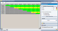
The SPC's [math]\displaystyle{ \alpha }[/math] value are set at 0.01 for the Critical Value and 0.1 for the Caution Value. When analyzed and color coded in Weibull++ the following window is obtained:
Here the Nov. 05 and Mar 06 sales periods are colored in yellow indicating that they are `outlier' sales periods, while the rest are green. One suspected reason for the variation may be the material used in production in this period. Further analysis confirmed that for these periods the material was acquired from a different supplier. This then implies that the units are not homogenous, and that there are different subpopulations present in the field populations.
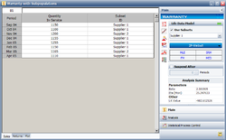
Based on this, the data is re-analyzed after categorizing the different shipments (using the ID column) based on their material supplier. The data as entered are shown next.
The new models that describe the data are (assuming a two-parameter Weibull distribution and using MLE as the analysis method for both sub-populations):
This analysis helped in uncovering different subpopulations as well as allowing us to compute different distributions for each subpopulation. Note that if the analysis were performed on the failure and suspension times in a regular Standard Folio, using the mixed Weibull distribution, one would not be able to detect which units fall into which subpopulation.

