Power Law Model Example: Difference between revisions
Kate Racaza (talk | contribs) No edit summary |
Lisa Hacker (talk | contribs) No edit summary |
||
| Line 1: | Line 1: | ||
<noinclude>{{Banner RGA Examples}}{{Navigation box}} | <noinclude>{{Banner RGA Examples}}{{Navigation box}} | ||
''These examples appear in the [ | ''These examples appear in the [https://help.reliasoft.com/reference/reliability_growth_and_repairable_system_analysis Reliability growth reference]''. | ||
</noinclude> | </noinclude> | ||
Latest revision as of 21:15, 18 September 2023
 |
New format available! This reference is now available in a new format that offers faster page load, improved display for calculations and images and more targeted search.
As of January 2024, this Reliawiki page will not continue to be updated. Please update all links and bookmarks to the latest references at RGA examples and RGA reference examples.
These examples appear in the Reliability growth reference.
Parameter Estimation Example
For the data in the following table, the starting time for each system is equal to 0 and the ending time for each system is 2,000 hours. Calculate the maximum likelihood estimates [math]\displaystyle{ \widehat{\lambda }\,\! }[/math] and [math]\displaystyle{ \widehat{\beta }\,\! }[/math].
| Repairable System Failure Data | ||
| System 1 ( [math]\displaystyle{ {{X}_{i1}}\,\! }[/math] ) | System 2 ( [math]\displaystyle{ {{X}_{i2}}\,\! }[/math] ) | System 3 ( [math]\displaystyle{ {{X}_{i3}}\,\! }[/math] ) |
|---|---|---|
| 1.2 | 1.4 | 0.3 |
| 55.6 | 35.0 | 32.6 |
| 72.7 | 46.8 | 33.4 |
| 111.9 | 65.9 | 241.7 |
| 121.9 | 181.1 | 396.2 |
| 303.6 | 712.6 | 444.4 |
| 326.9 | 1005.7 | 480.8 |
| 1568.4 | 1029.9 | 588.9 |
| 1913.5 | 1675.7 | 1043.9 |
| 1787.5 | 1136.1 | |
| 1867.0 | 1288.1 | |
| 1408.1 | ||
| 1439.4 | ||
| 1604.8 | ||
| [math]\displaystyle{ {{N}_{1}}=9\,\! }[/math] | [math]\displaystyle{ {{N}_{2}}=11\,\! }[/math] | [math]\displaystyle{ {{N}_{3}}=14\,\! }[/math] |
Solution
Because the starting time for each system is equal to zero and each system has an equivalent ending time, the general equations for [math]\displaystyle{ \widehat{\beta }\,\! }[/math] and [math]\displaystyle{ \widehat{\lambda }\,\! }[/math] reduce to the closed form equations. The maximum likelihood estimates of [math]\displaystyle{ \hat{\beta }\,\! }[/math] and [math]\displaystyle{ \hat{\lambda }\,\! }[/math] are then calculated as follows:
- [math]\displaystyle{ \widehat{\beta }= \frac{\underset{q=1}{\overset{K}{\mathop{\sum }}}\,{{N}_{q}}}{\underset{q=1}{\overset{K}{\mathop{\sum }}}\,\underset{i=1}{\overset{{{N}_{q}}}{\mathop{\sum }}}\,\ln (\tfrac{T}{{{X}_{iq}}})} = 0.45300 }[/math]
- [math]\displaystyle{ \widehat{\lambda }= \frac{\underset{q=1}{\overset{K}{\mathop{\sum }}}\,{{N}_{q}}}{K{{T}^{\beta }}} = 0.36224 \,\! }[/math]
The system failure intensity function is then estimated by:
- [math]\displaystyle{ \widehat{u}(t)=\widehat{\lambda }\widehat{\beta }{{t}^{\widehat{\beta }-1}},\text{ }t\gt 0\,\! }[/math]
The next figure is a plot of [math]\displaystyle{ \widehat{u}(t)\,\! }[/math] over the period (0, 3000). Clearly, the estimated failure intensity function is most representative over the range of the data and any extrapolation should be viewed with the usual caution.

Confidence Bounds
Using the data from the power law model example given above, calculate the mission reliability at [math]\displaystyle{ t=2000\,\! }[/math] hours and mission time [math]\displaystyle{ d=40\,\! }[/math] hours along with the confidence bounds at the 90% confidence level.
Solution
The maximum likelihood estimates of [math]\displaystyle{ \widehat{\lambda }\,\! }[/math] and [math]\displaystyle{ \widehat{\beta }\,\! }[/math] from the example are:
- [math]\displaystyle{ \begin{align} \widehat{\beta }= & 0.45300 \\ \widehat{\lambda }= & 0.36224 \end{align}\,\! }[/math]
The mission reliability at [math]\displaystyle{ t=2000\,\! }[/math] for mission time [math]\displaystyle{ d=40\,\! }[/math] is:
- [math]\displaystyle{ \begin{align} \widehat{R}(t)= & {{e}^{-\left[ \lambda {{\left( t+d \right)}^{\beta }}-\lambda {{t}^{\beta }} \right]}} \\ = & 0.90292 \end{align}\,\! }[/math]
At the 90% confidence level and [math]\displaystyle{ T=2000\,\! }[/math] hours, the Fisher matrix confidence bounds for the mission reliability for mission time [math]\displaystyle{ d=40\,\! }[/math] are given by:
- [math]\displaystyle{ CB=\frac{\widehat{R}(t)}{\widehat{R}(t)+(1-\widehat{R}(t)){{e}^{\pm {{z}_{\alpha }}\sqrt{Var(\widehat{R}(t))}/\left[ \widehat{R}(t)(1-\widehat{R}(t)) \right]}}}\,\! }[/math]
- [math]\displaystyle{ \begin{align} {{[\widehat{R}(t)]}_{L}}= & 0.83711 \\ {{[\widehat{R}(t)]}_{U}}= & 0.94392 \end{align}\,\! }[/math]
The Crow confidence bounds for the mission reliability are:
- [math]\displaystyle{ \begin{align} {{[\widehat{R}(t)]}_{L}}= & {{[\widehat{R}(\tau )]}^{\tfrac{1}{{{\Pi }_{1}}}}} \\ = & {{[0.90292]}^{\tfrac{1}{0.71440}}} \\ = & 0.86680 \\ {{[\widehat{R}(t)]}_{U}}= & {{[\widehat{R}(\tau )]}^{\tfrac{1}{{{\Pi }_{2}}}}} \\ = & {{[0.90292]}^{\tfrac{1}{1.6051}}} \\ = & 0.93836 \end{align}\,\! }[/math]
The next two figures show the Fisher matrix and Crow confidence bounds on mission reliability for mission time [math]\displaystyle{ d=40\,\! }[/math].


Auto Transmission Example
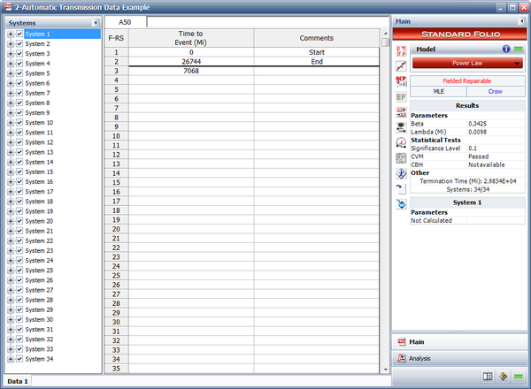
This case study is based on the data given in the article "Graphical Analysis of Repair Data" by Dr. Wayne Nelson [23]. The following table contains repair data on an automatic transmission from a sample of 34 cars. For each car, the data set shows mileage at the time of each transmission repair, along with the latest mileage. The + indicates the latest mileage observed without failure. Car 1, for example, had a repair at 7068 miles and was observed until 26,744 miles. Do the following:
- Estimate the parameters of the Power Law model.
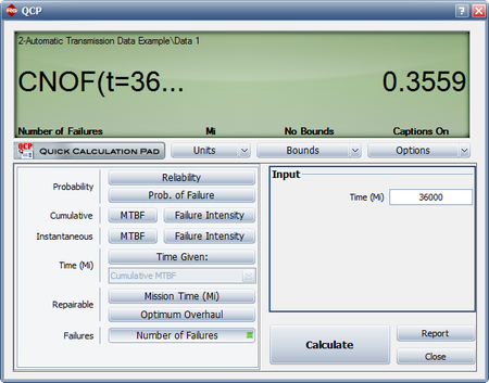
- Estimate the number of warranty claims for a 36,000 mile warranty policy for an estimated fleet of 35,000 vehicles.
| Automatic Transmission Data | ||||
| Car | Mileage | Car | Mileage | |
|---|---|---|---|---|
| 1 | 7068, 26744+ | 18 | 17955+ | |
| 2 | 28, 13809+ | 19 | 19507+ | |
| 3 | 48, 1440, 29834+ | 20 | 24177+ | |
| 4 | 530, 25660+ | 21 | 22854+ | |
| 5 | 21762+ | 22 | 17844+ | |
| 6 | 14235+ | 23 | 22637+ | |
| 7 | 1388, 18228+ | 24 | 375, 19607+ | |
| 8 | 21401+ | 25 | 19403+ | |
| 9 | 21876+ | 26 | 20997+ | |
| 10 | 5094, 18228+ | 27 | 19175+ | |
| 11 | 21691+ | 28 | 20425+ | |
| 12 | 20890+ | 29 | 22149+ | |
| 13 | 22486+ | 30 | 21144+ | |
| 14 | 19321+ | 31 | 21237+ | |
| 15 | 21585+ | 32 | 14281+ | |
| 16 | 18676+ | 33 | 8250, 21974+ | |
| 17 | 23520+ | 34 | 19250, 21888+ | |
Solution
- The estimated Power Law parameters are shown next.
- The expected number of failures at 36,000 miles can be estimated using the QCP as shown next. The model predicts that 0.3559 failures per system will occur by 36,000 miles. This means that for a fleet of 35,000 vehicles, the expected warranty claims are 0.3559 * 35,000 = 12,456.


Optimum Overhaul Example
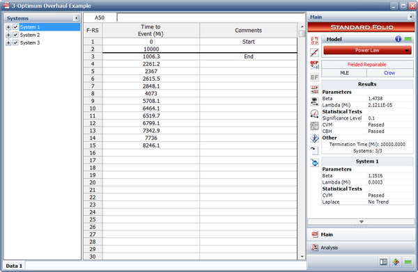
Field data have been collected for a system that begins its wearout phase at time zero. The start time for each system is equal to zero and the end time for each system is 10,000 miles. Each system is scheduled to undergo an overhaul after a certain number of miles. It has been determined that the cost of an overhaul is four times more expensive than a repair. The table below presents the data. Do the following:
- Estimate the parameters of the Power Law model.
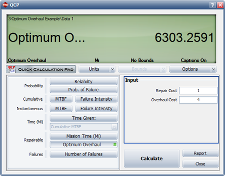
- Determine the optimum overhaul interval.
- If [math]\displaystyle{ \beta \lt 1\,\! }[/math], would it be cost-effective to implement an overhaul policy?
| Field Data | ||
| System 1 | System 2 | System 3 |
|---|---|---|
| 1006.3 | 722.7 | 619.1 |
| 2261.2 | 1950.9 | 1519.1 |
| 2367 | 3259.6 | 2956.6 |
| 2615.5 | 4733.9 | 3114.8 |
| 2848.1 | 5105.1 | 3657.9 |
| 4073 | 5624.1 | 4268.9 |
| 5708.1 | 5806.3 | 6690.2 |
| 6464.1 | 5855.6 | 6803.1 |
| 6519.7 | 6325.2 | 7323.9 |
| 6799.1 | 6999.4 | 7501.4 |
| 7342.9 | 7084.4 | 7641.2 |
| 7736 | 7105.9 | 7851.6 |
| 8246.1 | 7290.9 | 8147.6 |
| 7614.2 | 8221.9 | |
| 8332.1 | 9560.5 | |
| 8368.5 | 9575.4 | |
| 8947.9 | ||
| 9012.3 | ||
| 9135.9 | ||
| 9147.5 | ||
| 9601 | ||
Solution
- The next figure shows the estimated Power Law parameters.
- The QCP can be used to calculate the optimum overhaul interval, as shown next.
- Since [math]\displaystyle{ \beta \gt 1\,\! }[/math] the systems are wearing out and it would be cost-effective to implement an overhaul policy. An overhaul policy makes sense only if the systems are wearing out.

