Preventive Maintenance

Preventive maintenance (PM) is a schedule of planned maintenance actions aimed at the prevention of breakdowns and failures. The primary goal of preventive maintenance is to prevent the failure of equipment before it actually occurs. It is designed to preserve and enhance equipment reliability by replacing worn components before they actually fail. Preventive maintenance activities include equipment checks, partial or complete overhauls at specified periods, oil changes, lubrication and so on. In addition, workers can record equipment deterioration so they know to replace or repair worn parts before they cause system failure. Recent technological advances in tools for inspection and diagnosis have enabled even more accurate and effective equipment maintenance. The ideal preventive maintenance program would prevent all equipment failure before it occurs.

Value of Preventive Maintenance

There are multiple misconceptions about preventive maintenance. One such misconception is that PM is unduly costly. This logic dictates that it would cost more for regularly scheduled downtime and maintenance than it would normally cost to operate equipment until repair is absolutely necessary. This may be true for some components; however, one should compare not only the costs but the long-term benefits and savings associated with preventive maintenance. Without preventive maintenance, for example, costs for lost production time from unscheduled equipment breakdown will be incurred. Also, preventive maintenance will result in savings due to an increase of effective system service life.

Long-term benefits of preventive maintenance include:

• Improved system reliability.

• Decreased cost of replacement.

• Decreased system downtime.

• Better spares inventory management.

Long-term effects and cost comparisons usually favor preventive maintenance over performing maintenance actions only when the system fails.

When Does Preventive Maintenance Make Sense?

Preventive maintenance is a logical choice if, and only if, the following two conditions are met:

• Condition #1: The component in question has an increasing failure rate. In other words, the failure rate of the component increases with time, implying wear-out. Preventive maintenance of a component that is assumed to have an exponential distribution (which implies a constant failure rate) does not make sense!
  
• Condition #2: The overall cost of the preventive maintenance action must be less than the overall cost of a corrective action.
  

If both of these conditions are met, then preventive maintenance makes sense. Additionally, based on the costs ratios, an optimum time for such action can be easily computed for a single component. This is detailed in later sections.

The Fallacy of "Constant Failure Rate" and "Preventive Replacement"

Even though we alluded to the fact in the last section, it is important to make it explicitly clear that if a component has a constant failure rate (i.e., defined by an exponential distribution), then preventive maintenance of the component will have no effect on the component's failure occurrences. To illustrate this, consider a component with an [math]\displaystyle{ MTTF }[/math] = [math]\displaystyle{ 100 }[/math] hours, or [math]\displaystyle{ \lambda =0.01 }[/math], and with preventive replacement every 50 hours. The reliability vs. time graph for this case is illustrated in the following figure, where the component is replaced every 50 hours, thereby resetting the component's reliability to one. At first glance, it may seem that the preventive maintenance action is actually maintaining the component at a higher reliability.

However, consider the following cases for a single component:

Case 1: The component's reliability from 0 to 60 hours:

• With preventive maintenance, the component was replaced with a new one at 50 hours so the overall reliability is based on the reliability of the new component for 10 hours, [math]\displaystyle{ R(t=10)=90.48%\,\! }[/math], times the reliability of the previous component, [math]\displaystyle{ R(t=50)=60.65%\,\! }[/math]. The result is [math]\displaystyle{ R(t=60)=54.88%.\,\! }[/math]
  
• Without preventive maintenance, the reliability would be the reliability of the same component operating to 60 hours, or [math]\displaystyle{ R(t=60)=54.88%\,\! }[/math].
  

Case 2: The component's reliability from 50 to 60 hours:

• With preventive maintenance, the component was replaced at 50 hours, so this is solely based on the reliability of the new component for a mission of 10 hours, or [math]\displaystyle{ R(t=10)=90.48%\,\! }[/math].
  
• Without preventive maintenance, the reliability would be the conditional reliability of the same component operating to 60 hours, having already survived to 50 hours, or [math]\displaystyle{ {{R}_{C}}(T=60|50)=R(60)/R(50)=90.48%\,\! }[/math] .

As can be seen, both cases — with and without preventive maintenance — yield the same results.

Determining Preventive Replacement Time

As mentioned earlier, if the component has an increasing failure rate, then a carefully designed preventive maintenance program is beneficial to system availability. Otherwise, the costs of preventive maintenance might actually outweigh the benefits. The objective of a good preventive maintenance program is to either minimize the overall costs (or downtime, etc.) or meet a reliability objective. In order to achieve this, an appropriate interval (time) for scheduled maintenance must be determined. One way to do that is to use the optimum age replacement model, as presented next. The model adheres to the conditions discussed previously:

• The component is exhibiting behavior associated with a wear-out mode. That is, the failure rate of the component is increasing with time.

• The cost for planned replacements is significantly less than the cost for unplanned replacements.

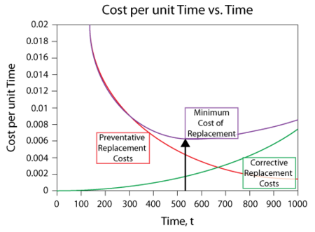
The following figure shows the Cost Per Unit Time vs. Time plot and it can be seen that the corrective replacement costs increase as the replacement interval increases. In other words, the less often you perform a PM action, the higher your corrective costs will be. Obviously, as we let a component operate for longer times, its failure rate increases to a point that it is more likely to fail, thus requiring more corrective actions. The opposite is true for the preventive replacement costs. The longer you wait to perform a PM, the less the costs; if you do PM too often, the costs increase. If we combine both costs, we can see that there is an optimum point that minimizes the costs. In other words, one must strike a balance between the risk (costs) associated with a failure while maximizing the time between PM actions.

Optimum Age Replacement Policy

To determine the optimum time for such a preventive maintenance action (replacement), we need to mathematically formulate a model that describes the associated costs and risks. In developing the model, it is assumed that if the unit fails before time [math]\displaystyle{ t\,\! }[/math] , a corrective action will occur and if it does not fail by time [math]\displaystyle{ t }[/math] , a preventive action will occur. In other words, the unit is replaced upon failure or after a time of operation, [math]\displaystyle{ t\,\! }[/math] , whichever occurs first. Thus, the optimum replacement time can be found by minimizing the cost per unit time, [math]\displaystyle{ CPUT\left( t \right).\,\! }[/math] [math]\displaystyle{ CPUT\left( t \right)\,\! }[/math] is given by:

[math]\displaystyle{ \begin{align} CPUT\left( t \right)= & \frac{\text{Total Expected Replacement Cost per Cycle}}{\text{Expected Cycle Length}} \\ = & \frac{{{C}_{P}}\cdot R\left( t \right)+{{C}_{U}}\cdot \left[ 1-R\left( t \right) \right]}{\mathop{}_{0}^{t}R\left( s \right)ds} \end{align} }[/math]

where:

• [math]\displaystyle{ R(t)\,\! }[/math] = reliability at time [math]\displaystyle{ t\,\! }[/math] .
  
• [math]\displaystyle{ {{C}_{P}}\,\! }[/math] = cost of planned replacement.
  
• [math]\displaystyle{ {{C}_{U}}\,\! }[/math] = cost of unplanned replacement.
  

The optimum replacement time interval, [math]\displaystyle{ t\,\! }[/math] , is the time that minimizes [math]\displaystyle{ CPUT\left( t \right).\,\! }[/math] This can be found by solving for [math]\displaystyle{ t\,\! }[/math] such that:

[math]\displaystyle{ \frac{\partial \left[ CPUT(t) \right]}{\partial t}=0 }[/math]

Or by solving for a [math]\displaystyle{ t\,\! }[/math] that satisfies the following equation:

[math]\displaystyle{ \frac{\partial \left[ \tfrac{{{C}_{P}}\cdot R\left( t \right)+{{C}_{U}}\cdot \left[ 1-R\left( t \right) \right]}{\mathop{}_{0}^{t}R\left( s \right)ds} \right]}{\partial t}=0 }[/math]

Interested readers can refer to Barlow and Hunter [2] for more details on this model.

Optimum Replacement Window in BlockSim 8

The Optimum Replacement window in BlockSim 8 is shown in the figure below.

Available Blocks

In BlockSim 7, optimum replacement calculations were performed for individual blocks. The utility in BlockSim 8 allows you to perform calculations either for an individual block or for multiple blocks in a diagram simultaneously. When working with multiple blocks, the calculations can be for individual blocks or for one or more groups of blocks.

If you are working with a diagram instead of with a single block, the Available Blocks area on the left side of the window lists all of the standard blocks (in RBDs) or the events (in fault trees), as well as the switches for any standby containers. The following requirements must be met for an item to be available for inclusion in the optimization calculations:

• Blocks must have a failure distribution.

• Switches must have a failure model assigned. Note that in the standby configuration, the switch is the item that is optimized, not the container or the contained blocks/dependent events.

• The failure model must meet the following requirements.

• Fixed reliability and exponential distributions are not allowed.

• Weibull distributions must have beta > 1.

• Gamma distributions must have k > 1.

• Loglogistic distributions must have std < 1.

• For generalized gamma distributions and mixed Weibull distributions, there must be an increasing failure rate within at least one time period. A local optimum can then be found within intervals with an increasing failure rate.

You can select an individual item's check box or drag the block into the table on the right side of the window to include the item in the optimization calculations. You can also select the check box in the Available Blocks header to select all check boxes. To remove items from the optimization calculations, you must clear the check box(es); you cannot drag items out of the table.

For each item that is included in the optimization calculations, you will need to specify the cost for a planned replacement and the cost for an unplanned replacement. This is done by calculating the costs for replacement based on the item settings using equations or simulation and then, if desired, manually entering any additional costs for either type of replacement in the corresponding columns of the table.

Estimate Costs

This calculates the costs of planned and unplanned tasks for each item based on its associated URD using the following equations.

• For the cost of planned tasks, here denoted as PM cost:

[math]\displaystyle{ \begin{align} \text{PM Cost}= \left(\text{PM Down Time Rate}+ \text{Block Level Down Time Rate} \right)\cdot \left( \text{MTTPM}+\text{Pool Delay} +\text{Crew Delay} \right) \\ + \text{Crew Labor Rate} \cdot \text{MTTPM} + \text{Cost per PM} + \text{Cost per Pool} +\text{Cost per Crew} \end{align} }[/math]

Notice: Only PM tasks based on item age are considered. If there is more than one PM task based on item age, only the first one is considered.

• For the cost of the unplanned task, here denoted as CM cost:

[math]\displaystyle{ \begin{align} \text{CM Cost}= \left(\text{CM Down Time Rate}+ \text{Block Level Down Time Rate} \right)\cdot \left( \text{MTTR}+\text{Pool Delay} +\text{Crew Delay} \right) \\ + \text{Crew Labor Rate} \cdot \text{MTTR} + \text{Cost per CM} + \text{Cost per Pool} +\text{Cost per Crew} \\ +\text{Block Level Cost per Failure} \end{align} }[/math]

The results will be used to populate the "Calculated Planned Replacement Cost" and "Calculated Unplanned Replacement Cost" columns.

Estimate Costs Using Simulation

This calculates the costs of planned and unplanned tasks for each item based on its associated URD using simulation. In other words, we run simulation for each item alone and estimate its costs. When you choose this command, a Simulation Settings window is shown, allowing you to specify the simulation settings. Once the simulation settings are specified, you can estimate the costs for each item using simulation.

The results will be used to populate the "Calculated Planned Replacement Cost" and "Calculated Unplanned Replacement Cost" columns.

Calculate

If you are working with a diagram instead of with a single block, when you click Calculate, you can choose from the following options:

• Calculate the individual optimum replacement time for each item.
• Calculate a common optimum replacement time, which is the most cost-effective time to replace all of the selected items concurrently.
• Calculate clustered optimum replacement times, which allows you to specify a number of times to replace groups of the selected items. For example, if you enter 3 in the Number of clusters field, the software will determine the three best times to replace groups of items such that all of the selected items are replaced at one of the three times.

If you are working with a single block, no choice is necessary. BlockSim will calculate the optimum replacement time for the items based on their failure characteristics and on the defined costs. This value will be displayed in the Optimum Replacement Time column of the table. In addition, the Cost per Unit Time column will display the estimated cost per unit time for a replacement performed at the calculated optimum replacement time. Multiply the replacement time by the cost per unit time to obtain the cost of replacing the item at the optimum replacement time

Cost vs. Time Plot

Choosing this command shows a plot of the results. If you have calculated individual optimum replacement times, the plot will show the cost for each item as a function of time. If you have calculated a common optimum replacement time, the plot will show the common cost as a function of time. If you have calculated clustered optimum replacement times, the plot will show the cost for each cluster as a function of time.

Create Maintenance Task(s) at Replacement Time

This enable you to create a preventive task for one or more of the items. The window that appears allows you to select which items to create tasks for. The preventive tasks created in this way restore the item to as good as new condition and are scheduled at fixed intervals based on item age, equal to the optimum replacement time.

Example: Optimum Replacement Time

The failure distribution of a component is described by a 2-parameter Weibull distribution with [math]\displaystyle{ \beta = 2.5\,\! }[/math] and [math]\displaystyle{ \eta = 1,000\,\! }[/math] hours.

• The cost for a corrective replacement is $5.
  
• The cost for a preventive replacement is $1.
  

Estimate the optimum replacement age in order to minimize these costs.

Solution

Prior to obtaining an optimum replacement interval for this component, the assumptions of the following equation must be checked.

[math]\displaystyle{ \begin{align} CPUT\left( t \right)= & \frac{\text{Total Expected Replacement Cost per Cycle}}{\text{Expected Cycle Length}} \\ = & \frac{{{C}_{P}}\cdot R\left( t \right)+{{C}_{U}}\cdot \left[ 1-R\left( t \right) \right]}{\mathop{}_{0}^{t}R\left( s \right)ds} \end{align} }[/math]

The component has an increasing failure rate, since it follows a Weibull distribution with [math]\displaystyle{ \beta \,\! }[/math] greater than 1. Note that if [math]\displaystyle{ \beta =1\,\! }[/math] , then the component has a constant failure rate and if [math]\displaystyle{ \beta \lt 1\,\! }[/math] , it has a decreasing failure rate. If either of these cases exist, then preventive replacement is unwise. Furthermore, the cost for preventive replacement is less than the corrective replacement cost. Thus, the conditions for the optimum age replacement policy have been met.

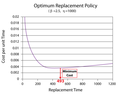
Using BlockSim, the failure parameters can be entered in the component's Block Properties window. You can then open the Optimum Replacement window and enter the costs (note that here we have to enter the costs, $1 and $5, in the "Additional Planned Replacement Cost" and "Additional Unplanned Replacement Cost" columns respectively) and compute the optimum time, [math]\displaystyle{ 493.0470 }[/math] .

The figure below shows a plot illustrating the cost per unit time.

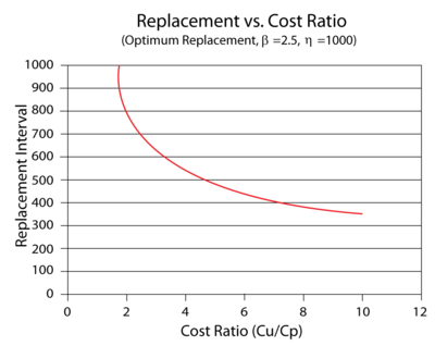
The effect of the corrective/preventive cost ratio on the optimum replacement interval is plotted in the following figure. It can be seen that as the cost ratio increases, the optimum replacement interval decreases. This is an expected result because the corrective replacement costs are much greater than the preventive replacement costs. Therefore, it becomes more cost-effective to replace the component more frequently before it fails.