Reliability Phase Diagrams (RPDs): Difference between revisions
Cruz Daniel (talk | contribs) mNo edit summary |
|||
| Line 17: | Line 17: | ||
In this figure, the taxiing, take-off, cruising and landing blocks represent the operational phases and the final block is a maintenance phase. Each of the operational phases in this diagram has two paths leading from it: a success path and a failure path. This graphically illustrates the consequences in each case. For instance, if the first taxiing phase is successful, the airplane will proceed to the take-off phase; if it is unsuccessful, the airplane will be sent for maintenance. The failure paths for the take-off, cruising and landing phases point to stop blocks, which indicate that the simulation of the mission ends. For the final taxiing phase, both the success and failure paths lead to the maintenance path; the node block allows you to model this type of shared outcome. | In this figure, the taxiing, take-off, cruising and landing blocks represent the operational phases and the final block is a maintenance phase. Each of the operational phases in this diagram has two paths leading from it: a success path and a failure path. This graphically illustrates the consequences in each case. For instance, if the first taxiing phase is successful, the airplane will proceed to the take-off phase; if it is unsuccessful, the airplane will be sent for maintenance. The failure paths for the take-off, cruising and landing phases point to stop blocks, which indicate that the simulation of the mission ends. For the final taxiing phase, both the success and failure paths lead to the maintenance path; the node block allows you to model this type of shared outcome. | ||
The execution of a phase diagram from its first phase to its last phase is referred to as one cycle. For example, for the airplane mentioned above, a single mission from the initial taxiing through the post-flight maintenance is one cycle. If the simulation end time exceeds the total duration of one cycle of a phase diagram, the simulation continues and the phase diagram is executed multiple times until the simulation end time is reached. Execution of a phase diagram multiple times during a simulation is referred to as cycling. During cycling, the age of components accumulated in the last phase of the previous cycle is carried over to the first phase of the next cycle | The execution of a phase diagram from its first phase to its last phase is referred to as one cycle. For example, for the airplane mentioned above, a single mission from the initial taxiing through the post-flight maintenance is one cycle. If the simulation end time exceeds the total duration of one cycle of a phase diagram, the simulation continues and the phase diagram is executed multiple times until the simulation end time is reached. Execution of a phase diagram multiple times during a simulation is referred to as cycling. During cycling, the age of components accumulated in the last phase of the previous cycle is carried over to the first phase of the next cycle. In summary, cycling is used to model the continuous operation of a system involving repetition of the same phases in the same sequence (e.g., an airplane making multiple flights). | ||
The sections that follow describe the types of phase blocks and other blocks that can be used in a phase diagram, as well as how those blocks can be connected. A more detailed example is then presented, followed by a discussion of the rules and assumptions that apply in phase diagram simulation. Finally, throughput in phase diagrams is discussed. | The sections that follow describe the types of phase blocks and other blocks that can be used in a phase diagram, as well as how those blocks can be connected. A more detailed example is then presented, followed by a discussion of the rules and assumptions that apply in phase diagram simulation. Finally, throughput in phase diagrams is discussed. | ||
Latest revision as of 14:21, 30 April 2021

The term phase diagram is used in many disciplines with different meanings. In physical chemistry, mineralogy and materials science, a phase diagram is a type of graph used to show the equilibrium conditions among the thermodynamically-distinct phases. In mathematics and physics, a phase diagram is used as a synonym for a phase space. In reliability engineering, we introduce the term phase diagram, or more specifically Reliability Phase Diagram or RPD, as an extension of the reliability block diagram (RBD) approach to graphically describe the sequence of different operational and/or maintenance phases experienced by a system. Whereas a reliability block diagram (RBD) is used to analyze the reliability of a system with a fixed configuration, a phase diagram can be used to represent/analyze a system whose reliability configuration and/or other properties change over time. In other words, during a mission the system may undergo changes in its reliability configuration (RBD), available resources or the failure, maintenance and/or throughput properties of its individual components. Examples of this include:
- Systems whose components exhibit different failure distributions depending on changes in the stress on the system.
- Systems or processes requiring different equipment to function over a cycle, such as start-up, normal production, shut-down, scheduled maintenance, etc.
- Systems whose RBD configuration changes at different times, such as the RBD of the engine configuration on a four-engine aircraft during taxi, take-off, cruising, and landing.
- Systems with different types of machinery operating during day and night shifts and with different amounts of throughput during each shift.
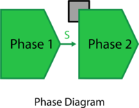
To analyze such systems, each stage during the mission can be represented by a phase whose properties are inherited from an RBD corresponding to that phase's reliability configuration, along with any associated resources of the system during that time. A phase diagram is then a series of such phases drawn (connected) in a sequence signifying a chronological order.
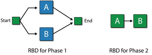
To better illustrate this, consider the four-engine aircraft mentioned previously. Assume that when a critical failure (system failure) occurs during taxiing, the airplane does not take off and is sent for maintenance instead. However, when a critical failure occurs during take-off, cruising, landing, the system is assumed to be lost. Furthermore, assume that the taxi phase requires only one engine, the take-off phase requires all four engines, the cruising phase requires any three of the four engines and the landing phase requires any two of the four engines. To model this, each one of these cases would require a different k-out-of-n redundancy on the engines and thus a different RBD. Creating an RBD for each phase is trivial. However, what you need is a way to transition from one RBD to the next, in a specified sequence, while maintaining all the past history of each component during the transition.
In other words, a new engine would transition to the take-off phase with an age equal to the time it was used during taxi, or an engine that failed while in flight would remain failed in the next phase (i.e., landing). To model this, a block for each phase would be used in the phase diagram, and each phase block would be linked to the appropriate RBD. This is illustrated in the figure below.

In this figure, the taxiing, take-off, cruising and landing blocks represent the operational phases and the final block is a maintenance phase. Each of the operational phases in this diagram has two paths leading from it: a success path and a failure path. This graphically illustrates the consequences in each case. For instance, if the first taxiing phase is successful, the airplane will proceed to the take-off phase; if it is unsuccessful, the airplane will be sent for maintenance. The failure paths for the take-off, cruising and landing phases point to stop blocks, which indicate that the simulation of the mission ends. For the final taxiing phase, both the success and failure paths lead to the maintenance path; the node block allows you to model this type of shared outcome.
The execution of a phase diagram from its first phase to its last phase is referred to as one cycle. For example, for the airplane mentioned above, a single mission from the initial taxiing through the post-flight maintenance is one cycle. If the simulation end time exceeds the total duration of one cycle of a phase diagram, the simulation continues and the phase diagram is executed multiple times until the simulation end time is reached. Execution of a phase diagram multiple times during a simulation is referred to as cycling. During cycling, the age of components accumulated in the last phase of the previous cycle is carried over to the first phase of the next cycle. In summary, cycling is used to model the continuous operation of a system involving repetition of the same phases in the same sequence (e.g., an airplane making multiple flights).
The sections that follow describe the types of phase blocks and other blocks that can be used in a phase diagram, as well as how those blocks can be connected. A more detailed example is then presented, followed by a discussion of the rules and assumptions that apply in phase diagram simulation. Finally, throughput in phase diagrams is discussed.
Phase Blocks
Operational Phases
In RPDs, two types of phases are used: operational phases and maintenance phases. An operational phase is used to represent any stage of the system's mission that is not exclusively dedicated to the execution of maintenance tasks. Operational phases are always defined by (linked to) an RBD. Each operational phase has a fixed, predefined time duration.
Operational Phase Properties
Diagram The diagram property is used to associate an RBD with a phase. You can select and associate any existing simulation RBD with a phase. Note that common components across different RBDs are identified by name. In other words, a component with the exact same name in two RBDs is assumed to be the same component working in two different phases.
Phase Duration The duration of an operational phase is fixed and needs to be specified. However, this duration may be affected by the choice of path you choose followed by this phase. If a failure has not occurred by the end of the specified phase duration, the simulation will proceed along the success path leading from the phase block. If a failure occurs, the simulation will proceed along the failure path leading from the phase block.
Phase Duty Cycle This property allows you to specify a common duty cycle value for the entire RBD that the phase represents, thereby modeling situations where the actual usage of the RBD during system operation is not identical to the usage for which you have data (either from testing or from the field). This can include situations where the item:
- Does not operate continuously (e.g., a DVD drive that was tested in continuous operation, but in actual use within a computer accumulates only 18 minutes of usage for every hour the computer operates).
- Is subjected to loads that are greater than or less than the rated loads (e.g., a motor that is rated to operate at 1,000 rpm but is being used at 800 rpm).
- Is affected by changes in environmental stress (e.g., a laptop computer that is typically used indoors at room temperature, but is being used outdoors in tropical conditions).
In these cases, continuous operation at the rated load is considered to be a duty cycle of 1. Any other level of usage is expressed as a percentage of the rated load value or operating time. For example, consider the DVD drive mentioned above; its duty cycle value would be 18 min / 60 min = 0.3. A duty cycle value higher than 1 indicates a load in excess of the rated value.
If a duty cycle is specified for the phase and there are also duty cycles specified for blocks within the RBD, their effects are compounded. For instance, consider the aircraft example given earlier. During the take-off phase, the subsystems experience 1.5 times the normal stress, so you would use a phase duty cycle value of 1.5. We also know that the landing gear is not used continuously during take-off. Assume that the landing gear is actually in use only 30% of the time during take-off. Each landing gear block in the RBD, then, would have a duty cycle value of 0.3. For each block, the effects of the phase duty cycle and the block duty cycle are compounded, yielding an effective duty cycle value of 1.5 x 0.3 = 0.45.
Maintenance Phases
A maintenance phase represents the portion of a system's mission time where the system is down and maintenance actions are performed on some or all of its components. For representation ease a maintenance phase is defined by (linked to) a maintenance template. This template can be thought of as a list, or a collection, of the specific components (blocks) that are designated to undergo inspection, repair or replacement actions during the maintenance phase, along with their maintenance priority order. In other words, if blocks A, B and C are to undergo maintenance during a specific phase, they are placed in a maintenance template in a priority sequence. Depending on the resources available, the actions are prioritized as resources permit. That is, if three repair crews were available along with three spare parts, actions on A, B and C would be carried out simultaneously. However, if only one crew was available, the actions would be carried out based on the priority order defined in the template. Given that all aspects of maintenance can be probabilistically defined, the duration of a maintenance phase, unlike an operational phase, is not fixed and the phase lasts as long as it takes to complete all actions specified in the phase. To illustrate this, consider a race car that competes in two races, and even though corrective repair actions can be done during each race as needed, the race car then undergoes a major overhaul (i.e., series of maintenance actions). For this example assume the major sub-systems of the car undergoing these maintenance tasks are the engine, the transmission, the suspension system and the tires. The operation of the race car can then be represented as a phase diagram consisting of two operational phases, representing the two races, and one maintenance phase representing the maintenance activities. The figure below shows such a phase diagram along with the maintenance template.

Maintenance Phase Properties
Maintenance Template
This specifies the maintenance template to be used in the currently selected maintenance phase.
Interval Maintenance Threshold
The Interval Maintenance Threshold property provides the ability to add some flexibility to the timing of scheduled maintenance tasks. In other words, tasks based on system or item age intervals (fixed or dynamic) will be performed if the start of the maintenance phase is within (1-X)% of the scheduled time for the action. It is used to specify an age interval when a maintenance task will be performed. This helps in optimizing the resources allocated to repair the system during a maintenance phase by performing preventive maintenance actions or inspections when the system is already down in a maintenance phase. For example, a preventive maintenance action is scheduled for a car (e.g., an oil change, tire rotation, etc.) every 60,000 miles, but a system downing failure of an unrelated component occurs at 55,000 miles. Here the system age threshold will determine whether the preventive maintenance will be performed earlier than scheduled. If the Interval Maintenance Threshold is 0.9, the preventive maintenance will be performed since the failure occurred after the system accumulated 91.67% of the time to the scheduled maintenance or is within 8.33%, (60,000-55,000)/60,000= 8.33%, of the system age at which the preventive maintenance was originally scheduled. If the system age threshold was 0.95, the preventive maintenance will not be performed at 55,000 miles, since the system failure did not occur within 5% of the system age at which the preventive maintenance was originally scheduled (1-0.95=0.05 or 5%).
For example, consider a system that has two components: Block A and Block B. The system undertakes a mission that can be divided into two phases. The first phase is an operational phase with a duration of 1,370 hours, with both the components in a parallel configuration. In this phase, Block A fails every 750 hours while Block B fails every 1,300 hours. Corrective maintenance on Block A in this phase requires 100 hours to be completed. A preventive maintenance of 20 hours duration also occurs on Block A every 500 hours. No maintenance can be carried out on Block B in this phase.
The second phase of the mission is a maintenance phase. In this phase, Block A has the same maintenance actions as those in the first phase. A corrective maintenance of 100 hours duration is defined for Block B. Phase 2 also has a value of 0.70 set for the Interval Maintenance Threshold. All maintenance actions during the entire mission of the system have a type II restoration factor of 1.
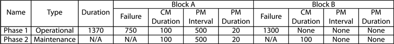
The system behavior from 0 to 3,500 hours is shown in the plot below and described next.
- Phase 1 begins at time 0 hours. The duration of this phase is 1,370 hours.
- At 500 hours, the first of the scheduled PMs for Block A begins. The duration of these maintenance tasks is 20 hours. The scheduled maintenance ends at 520 hours.
- At 1,000 hours, another PM occurs for Block A based on the set policy. This maintenance ends at 1,020 hours.
- At 1,300 hours, Block B fails after accumulating an age of 1,300 hours. A system failure does not occur because Block B is in a parallel configuration with Block A in this phase. Repairs for Block B are not defined in this phase. As a result Block B remains in a failed state.
- At 1,370 hours, phase 1 ends and phase 2 begins. Phase 2 is a maintenance phase. Block B is repairable in this phase and has a CM duration of 100 hours. As a result, repairs on Block B begin and are completed at 1,470 hours. Block A has the next PM scheduled to occur at 1,500 hours. However, phase 2 has an Interval Maintenance Threshold of 0.7 for Preventive and Inspection Policies. The time remaining to the next PM is 130 hours (1,500-1,370 = 130 hours). This remaining time over the PM policy time of 500 hours is 26%. This is within 0.3 (1-0.70 = 0.3) or 30% corresponding to the threshold value of 0.70. Thus the PM task that is to occur at 1,500 hours is carried out in the maintenance phase from 1,370 hours to 1,390 hours, while no PM occurs at 1,500 hours. All maintenance actions are completed by 1,470 hours and phase 2 ends at this time. This completes the first cycle of operation for the phase diagram.
- At 1,470 hours, phase 1 begins in the second cycle.
- At 2,000 hours, the next PM for Block A begins. This maintenance ends at 2,020 hours.
- At 2,500 hours, another PM is carried out on Block A and is completed by 2,520 hours.
- At 2,770 hours, Block B fails in the second cycle of phase 1 after accumulating an age of 1,300 hours. Since no repair is defined for the block in this phase, it remains in a failed state.
- At 2,840 hours, phase 1 completes its duration of 1,370 hours and ends. Phase 2 begins in the second cycle and the corrective maintenance, defined for a duration of 100 hours for Block B, begins. This repair action ends at 2,940 hours. For Block A, the time remaining until the next PM at 3,000 hours is 160 hours (3000-2840 = 160 hours). This remaining time over the PM policy of 500 hours is 32%. This is not within 30% corresponding to the threshold value of 0.70. Thus the PM due at 3,000 hours is not considered close enough to the beginning of the maintenance phase and is not carried out in this phase. At 2,940 hours, all maintenance actions are completed in phase 2 and phase 2 ends. This also completes the second cycle of operation for the phase diagram.
- At 2,940 hours, phase 1 begins in the third cycle.
- At 3,000 hours, the scheduled maintenance on Block A occurs. This PM ends at 3,020 hours.
- At 3,500 hours, the simulation ends.
Success/Failure Paths
For a failure path, on system failure, the system goes to somewhere immediately when the failure occurs. For a success path, if there is no system failure during this phase, the system goes to somewhere by the end of the current phase.
In BlockSim 7, there was only one path from each phase. The failure outcome for each phase was defined via a drop-down list. The success and failure paths used in BlockSim 8 and above make it easy to see what will happen upon success or failure for each block. They also allow you to create more complex phase diagrams, in which success and failure may lead to entirely different sets of phases. In addition, they offer an additional possible outcome of failure. Previously, the outcome of failure could be maintenance, stopping the simulation or continuing the simulation; now another possible outcome of failure can be continuing simulation on a different path.
For example, consider a system whose RBDs for Phase 1 and Phase 2 are as shown in the figure below:
In Phase 1, Block A follows Weibull distribution with Beta = 1.5 and Eta = 1000 hours. Block B follows Weibull distribution with Beta = 1.5 and Eta = 1200 hours. No maintenance.
In Phase 2, Block A follows Weibull distribution with Beta = 1.5 and Eta = 900 hours. Block B follows Weibull distribution with Beta = 1.5 and Eta = 1150 hours. No maintenance.
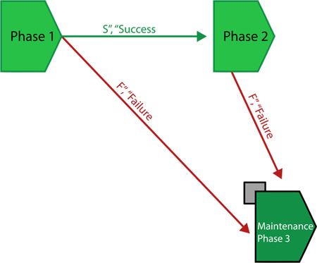
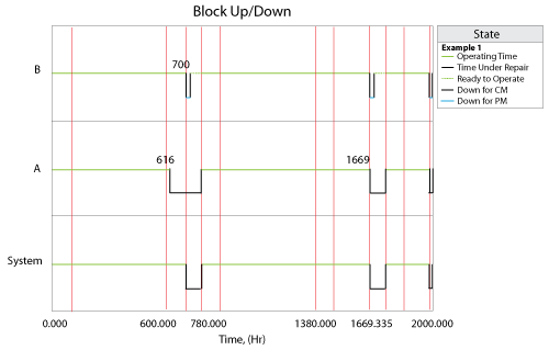
Scenario 1
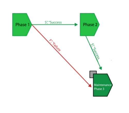
Suppose the phase diagram is as shown next. The maintenance phase has a CM with duration 80 hours and PM with duration 20 hours for both Block A and B. Phase 1 has a duration 100 hours and Phase 2 has a duration 500 hours. If there is no failure in Phase 1, upon finish, it goes to Phase 2. If there is a failure in Phase 1, it would immediately go to Maintenance Phase 3. If there is no failure in Phase 2, upon finish, it goes back to Phase 1. If there is a failure in Phase 2, it would immediately go to Maintenance Phase 3.
The Block Up/Down plot is shown below:
- At the first cycle (0-100 hours for Phase 1 and 200-600 hours for Phase 2), there is no failure, thus after Phase 2, Phase 1 is executed (back to Phase 1 after this cycle).
- At 616 hours (Phase 1 of the second cycle), Block A fails. The system doesn't enter Maintenance Phase 3 immediately because in Phase 1, Block A and Block B are parallel. Failure of only Block A does not bring the system down.
- At 700 hours, after Phase 1, the system goes into Phase 2. In Phase 2, the failure of Block A (passed from Phase 1) brings the system down because in Phase 2, Block A is in series with Block B. Thus the system goes into Maintenance Phase 3 immediately. Block B is not down, thus it gets PM with duration 20 hours. Block A gets CM with duration 100 hours.
- At 1669 hours, Block A fails in Phase 2, which brings down the system and the system goes into Maintenance Phase 3 immediately. Block A gets CM and Block B gets PM.
Scenario 2
Now suppose that the phase diagram is as follows, where everything is the same as in Example 1 except that the path from Phase 2 to Maintenance Phase 3 changes from a failure path to a success path. This means that whether or not there is a failure in Phase 2, the system would go to the Maintenance Phase 3 after Phase 2. But if there is a failure in Phase 2, the system would go to the Maintenance Phase 3 after Phase 2, not immediately.
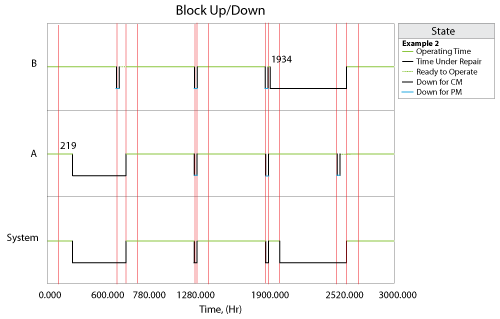
The Block Up/Down plot is shown below:
- At 219 hours, Block A fails in Phase 2. This failure brings the system down. However, since the path from Phase 2 to Maintenance Phase 3 is a success path, the system doesn't go into Maintenance Phase 3 immediately. Instead, it goes into Maintenance Phase 3 after Phase 2 ends. Block A gets CM and Block B gets PM in the maintenance phase.
- At 1934 hours, Block B fails in Phase 1. This failure doesn't bring the system down because in Phase 1, the system is in parallel structure. After Phase 1, the system goes into Phase 2 and the failure of Block B brings they system down in Phase 2. However, the system doesn't go into Maintenance Phase 3 immediately because the path between them is a success path. The system goes into Maintenance Phase 3 after Phase 2 ends, and Block B gets CM and Block A gets PM there.
Node Blocks and Stop Blocks
Starting with Version 8, the two possible outcomes of an operational phase block are modeled using success and failure paths. Where previously a failure outcome was defined as part of the operational phase block's properties, it is now graphically represented within the diagram. Node blocks and stop blocks are provided to allow you to build configurations that are both accurate and readable.
Node Blocks
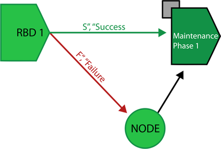
The purpose of a node block is simply to enable configurations that would otherwise not be possible due to limitations on connecting blocks. For example, consider an instance where maintenance is scheduled to be performed after the operational phase has completed successfully, and if a failure occurs during simulation, that maintenance will take place upon failure. In this case, the operational phase block's success and failure outcomes are identical. Success paths and failure paths cannot be identical in phase diagrams, however, so you would model this configuration in one of two ways:
- If the operational phase stops upon failure of the block and the simulation moves to the next phase along the success path, you would use a node block to model this configuration, as shown next.
- If the operational phase continues for the specified duration despite failure and the simulation then moves to the next phase along the success path, you would simply not create a failure path.
- If there is only one path, the success path observed for a phase, then on system failure at this phase, the "continue simulation" rule of BlockSim 7 applies. Under "continue simulation," when a system failure occurs, repairs begin as per the repair policy selected and the time to restore the system is part of the operational phase's time. In other words, the repairs continue in the operational phase until the system is up again. If the repairs are not completed before the phase ends, the repairs continue into the next phase. Thus, under this rule the duration of an operational phase is not affected by a system failure. As an example of this rule, consider a production line operating in two phases: a day shift and a night shift. A failure occurs in the day shift that renders the production line non-operational. Repair of the production line begins immediately and continues beyond the day shift. The production line is back up after midnight. In this case, the repair of the production line exhausts all of the duration of the day shift phase from the time of the failure to the end of the phase. Some part of the night shift phase is also exhausted.
Node blocks can have unlimited incoming connections and a single outgoing connection.
Stop Blocks
Stop blocks indicate that the simulation of the mission ends. A new simulation may then begin, if applicable. This is useful in situations where maintenance is not possible upon failure.
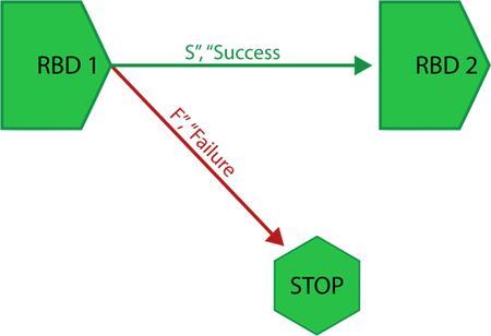
Stop blocks can have unlimited incoming connections. No outgoing connections can be defined for stop blocks.
When a path leads to a stop node, it is the same as the option "Start New Simulation" in BlockSim 7, which would halt the simulation and effectively means the end of the mission if the system fails. Specifically, if a failure path leads to a stop node the execution of the current operational phase and all phases that follow the current phase is halted, and the mission aborted. The stop node can be used to model a system whose failure cannot be repaired and the mission has to be aborted if a failure occurs. A good example of this would be the aircraft case discussed previously. A catastrophic failure during cruising would end the mission.
Subdiagram Phase Blocks
Subdiagram phase blocks represent other phase diagrams within the project. Using subdiagram phase blocks allows you to incorporate phase diagrams as phases within other phase diagrams. This allows you to break down extremely complex configurations into smaller diagrams, increasing understandability and ease of use and avoiding unnecessary repetition of elements.
Subdiagram phase blocks can have unlimited incoming connections and up to two outgoing connections, which may include one success path and one failure path. The success path and the failure path must be different; if both success and failure of the block actually lead to the same outcome, you can use a node block to model this configuration.
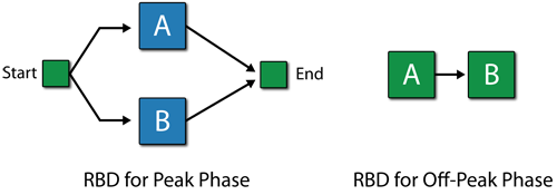
To illustrate how subdiagram blocks are handled in BlockSim’s simulations, consider a server that has two shifts each day, a day shift lasting 8 hours and a night shift lasting 16 hours. Within each shift, it has a peak period and an off-peak period with different durations.
The RBDs for the Peak phase and the Off-Peak phase are:
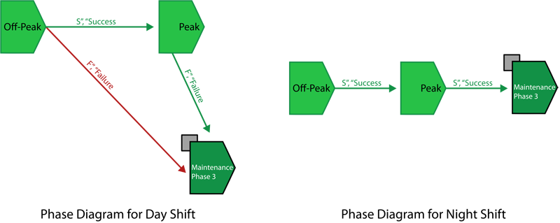
The phase diagrams for the Night Shift and Day Shift are:
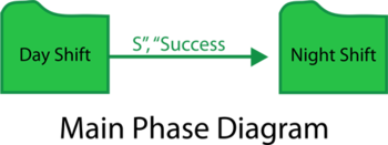
The main phase diagram with phase subdiagram blocks is:
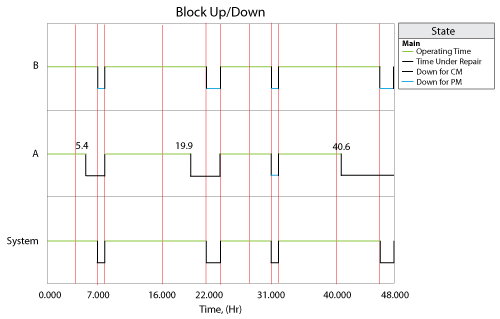
During the Peak phase, the reliability of Block A follows W(1.5,30) and the reliability of Block B follows W(1.5,40). During the Off-Peak phase, the reliability of Block A follows W(1.5,15) and the reliability of Block B follows W(1.5,20). In the Day Shift diagram, both blocks have CM and PM with duration = 1 hour; in the Night Shift diagram, both blocks have CM and PM with duration = 2 hours. In the Day Shift diagram, the duration of the Off-Peak phase is 4 hours and the duration of the Peak phase is 3 hours. In the Night Shift diagram, the duration of the Off-Peak phase is 8 hours and the duration of the Peak phase is 6 hours.
The system log for 2 days (48 hours) is shown in the figure below.
- At 5.4 hours, in the Peak phase of the Day Shift diagram, Block A fails. After this Peak phase, Block A gets CM and Block B gets PM in the maintenance phase.
- At 19.9 hours, in the Peak phase of the Night Shift diagram, Block A fails again. After this Peak phase, Block A gets CM and Block B gets PM in the maintenance phase.
- At 40.6 hours, in the Peak phase of the Night Shift diagram, Block A fails again. After this Peak phase, Block A gets CM and Block B gets PM in the maintenance phase.
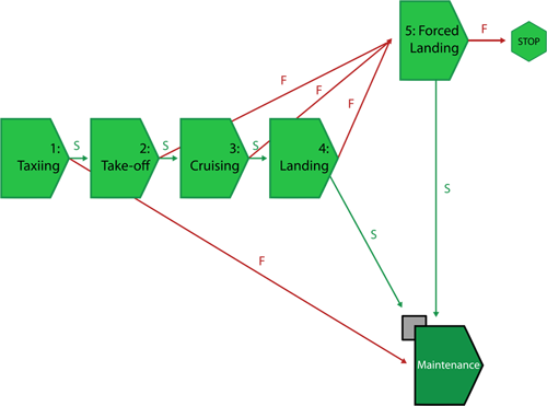
Example: Aircraft Phases with Forced Landing
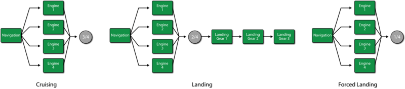
Consider simulating a flight mission for a four-engine aircraft. The configuration of the aircraft changes at different time. During the taxiing phase, the navigation system, one out of the four engines and all three landing gears are needed. During the take-off phase, all four engines, the navigation system and all three landing gears are needed. During the cruising phase, the navigation system and three of the four engines are required. During the landing phase, the navigation system, two of the four engines and all three landing gears are required. After finishing a journey with these four phases, the aircraft goes into a maintenance phase for maintenance. However, in addition to the four operational phases discussed, there is a special operational phase called the forced landing phase. This phase is used for modeling the case when there is a failure during take-off, cruising or landing phase, forcing the aircraft to land. If the forced landing succeeds, the aircraft goes into the maintenance phase. However, if the forced landing fails, the aircraft crashes and the simulation ends.
The purpose of this example is to illustrate how to create a nonlinear system with Failure/Success links in phase simulation.
RBDs and Phase Diagram
The RBDs for the Taxiing phase and the Take-Off phase are:
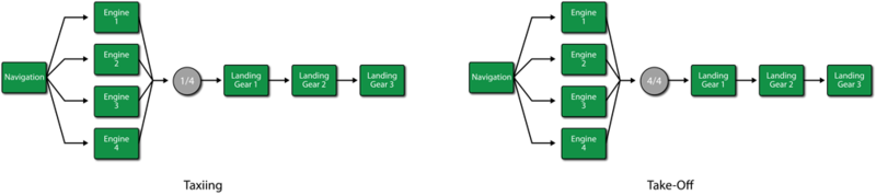
The RBDs for other three phases are:
The Phase diagram is:
The reliability of the navigation system follows a Weibull distribution with Beta=1.5 and Eta=30 hours. The reliability of the engines follows a Weibull distribution with Beta = 1.5 and Eta = 20 hours. The reliability of the landing gears follows a Weibull distribution with Beta = 1.5 and Eta = 15 hours.
In the maintenance phase, all blocks have CM with duration = 3 hours. CM is performed upon item failure. All blocks also are subjected to PM with duration = 0.5 hours and the PM is performed when the maintenance phase starts. Both CM and PM restore the blocks to as good as new.
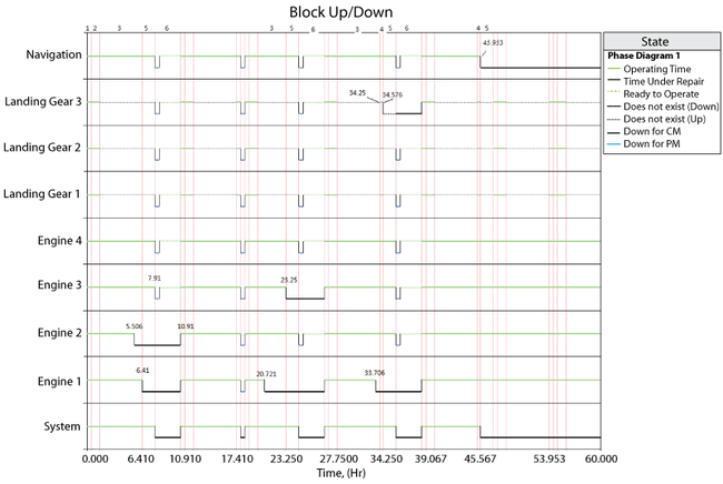
Block Up/Down plot
- At time 5.506 hours, in the Cruising phase, Engine 2 fails. However, this failure doesn't bring the system down because in the Cruising phase, only three of the four engines are required.
- At time 6.41 hours, in the Cruising phase, Engine 1 fails too. This failure brings the system down and the system goes into the Forced Landing phase immediately.
- At time 7.91 hours, the Forced Landing phase is done. No failure happened in this phase, which means the forced landing is successful. The system goes into the Maintenance phase. All blocks except Engine 1 and Engine 2 get PM in the Maintenance phase.
- At time 10.91 hours, Engine 1 and Engine 2 are done with their CM and the system goes back to the Taxiing phase.
- At time 20.721 hours, in the Cruising phase, Engine 1 fails again. Of course, this failure doesn't bring the system down.
- At time 23.25 hours, in the Cruising phase, Engine 3 fails and this failure brings the system down. The system goes into the Forced Landing phase. After the Forced Landing phase, the system goes into the Maintenance phase.
- At time 33.706 hours, in the Cruising phase, Engine 1 fails again. This failure doesn't bring the system down.
- At time 34.25 hours, the system goes into the Landing phase.
- At time 34.576 hours, in the Landing phase, Landing Gear 3 fails and this failure brings the system down. The system goes into the Forced Landing phase immediately.
- At time 45.953 hours, in the Landing phase, the navigation system fails. This failure brings the system down and the system goes into the Forced Landing phase immediately. In the Forced Landing phase, the navigation system is in series with other blocks, the failure of the navigation system brings the system down. Thus there is a system failure in the Forced Landing phase, which means the forced landing fails and the system goes into the Stop node. Simulation stops.
Simulation Rules and Assumptions
When Transferring Interrupted Maintenance Tasks Across Phases
Maintenance tasks in progress during one operational phase can be interrupted if that phase ends before the repair is completed. For example, a crew delay or spare parts order may extend the duration of a repair beyond the duration of the phase. As described next, the software handles these interruptions differently, based on the stage in which the repair was interrupted and whether or not the failed block is present in the next contiguous phase.
- 1. If a phase ends during the repair of a failed block and the block is present in the next contiguous phase:
- a) If the same task is present in both phases, then the task will continue as-is in the next phase. This is considered an uninterrupted event, and counts as a single unique event at both the block and the system level.
- b) If the interrupted task is not used in the next phase, then the task is cancelled and new tasks are applied as needed. In this case, all crew calls are cancelled and spare parts are restocked.
- 1) If the repair has started or the crew is delayed (crew logistic delay), the call will be assumed accepted and the component will be charged for it. If the crew was occupied with another component’s repair, the call will be assumed rejected and hence not charged to the component.
- 2) If the call for spare parts incurred emergency charges, those are charged to the block; otherwise, there are no other charges to the block.
- 1. If a phase ends during the repair of a failed block and the block is present in the next contiguous phase:
- 2. If a phase ends during the repair of a failed block and the block is not present in the next contiguous phase, then the task is cancelled and new tasks are applied as needed. All crew calls are cancelled and spare parts are restocked:
- a) If the repair has started or the crew is delayed (crew logistic delay), the call will be assumed accepted and the component will be charged for it. If the crew was occupied with another component’s repair, the call will be assumed rejected and hence not charged to the component.
- b) If the call for spare parts incurred emergency charges, those are charged to the block; otherwise, there are no other charges to the block.
- c) Discontinuous events are counted as two distinct events at both the block and the system level.
- d) When the system fails in a phase that has a failure path leading to a stop block, the system will remain down for the remainder of the simulation. From that point on, the blocks that are down are assumed unavailable and the blocks that are up are assumed operational for availability calculations.
- 2. If a phase ends during the repair of a failed block and the block is not present in the next contiguous phase, then the task is cancelled and new tasks are applied as needed. All crew calls are cancelled and spare parts are restocked:
For Stop Blocks
When a system failure occurs in a phase where the failure path points to a stop block, the simulation is aborted. Once this failure occurs, the following assumptions apply to the results:
- • Components that are under repair or maintenance remain down and unavailable for the rest of the simulation.
- • Components that are operating remain up for the rest of the simulation.
For a Maintenance Phase
A system is considered down and unavailable during the execution of a maintenance phase and remains down until all components have been repaired or maintained according to the properties specified for the maintenance phase. A maintenance phase is executed when the simulation reaches the phase while progressing through the phase diagram, either following a success path or a failure path. The following assumptions apply to both cases.
- 1. When a component enters a maintenance phase in a down state, the following rules apply:
- a) If a task is in progress for this component, the event will transfer to the maintenance phase provided that the same task is present in the maintenance phase. The rules for interrupted tasks apply as noted above.
- b) If the component is failed but no corrective maintenance is in progress (either because the component was non-repairable in the phase where it failed or because it had a task scheduled to be executed upon inspection and was waiting for an inspection), a repair is initiated according to the corrective maintenance properties specified for the component in the maintenance phase.
- c) Failed components are fixed in the order in which they failed.
- 2. When a component enters a maintenance phase in an operating state, the following rules apply:
- a) Maintenance will be scheduled as follows:
- 1) Tasks based on intervals or upon start of a maintenance phase
- 2) Tasks based on events in a maintenance group, where the triggering event applies to a block
- 3) Tasks based on system down
- 4) Tasks based on events in a maintenance group, where the triggering event applies to a subdiagram
- Within these categories, order is determined according to the priorities specified in the maintenance template (i.e., the higher the task is on the list, the higher the priority).
- a) Maintenance will be scheduled as follows:
- 1. When a component enters a maintenance phase in a down state, the following rules apply:
- b) An inspection or preventive task may be initiated, if applicable, with inspections taking precedence over preventive tasks. Inspections and/or preventive tasks are initiated if one of the following applies:
- 1) Upon certain events:
- a) The task is set to be performed when a maintenance phase starts.
- b) The policy is set to be performed based on events in a maintenance group and one of those events occurs within the one of the specified maintenance groups. Note that such a triggered maintenance does not follow the priorities specified in the maintenance template, but is sent to the end of the queue for repair.
- c) The task is set to be performed whenever the system is down.
- 2) At certain intervals:
- a) The task is set to be performed at a fixed time interval, based on either item age or calendar time, and the maintenance falls within the maintenance threshold specified in the maintenance phase.
- 1) Upon certain events:
- b) An inspection or preventive task may be initiated, if applicable, with inspections taking precedence over preventive tasks. Inspections and/or preventive tasks are initiated if one of the following applies:
- If the inspection task is not set to bring either the item or the system down, the inspection will still be considered a downing inspection.
Finally, if a block enters a maintenance phase in a failed state:
- 1. If the block does not have a corrective task in the maintenance phase but does have an on condition task, the preventive portion of the on condition task is triggered immediately in order to restore the block.
- 2. A maintenance phase will not end until all components are restored. Therefore, if any failed block does not have a task that restores it, the maintenance phase will not end.
Phase Throughput
Phase throughput is the maximum number of items that a system can process during a particular phase. It is defined at the phase level as a phase property in an operational phase. For a detailed discussion of throughput at the block level see Throughput Analysis. Phase throughput can be thought of as the initial throughput that enters the system. For example, imagine a textile factory that receives different quantities of raw materials during different seasons. These seasons could be treated as different phases. In this case a phase may be seen as sending a certain quantity of units to the first component of the system (the textile factory in this case). Depending on the capacity and availability of the factory, these units may be all processed or a backlog may accumulate.
Alternatively, phase throughput can be used as a constraint to the throughput of the system. An example would be the start up period in a processing plant. When the plant stops operating, the equipment requires a warm up period before reaching its maximum production capacity. In this case the phase throughput may be used to limit the capacity of the first component which in turn would limit the throughput of the rest of the system. Note that there is no phase-related backlog for this example. In BlockSim this can be modeled by checking the Ignore backlog option in the Block Properties window for the first component.
Phase throughput can be one of the following:
- Unrestricted throughput specifies that the amount of output the system can process during the phase will be equal to the amount that the linked diagram can process during the specified phase duration.
- Constant throughput allows you to specify an amount of throughput per unit time that is the same throughout the entire simulation.
- Variable throughput allows you to specify an amount of throughput per unit time that varies over the course of the simulation. For example, the flow of oil from a well may drop over time as the oil reserves are depleted so the amount of throughput per unit time will decrease as the simulation time increases.
Constant Throughput Example
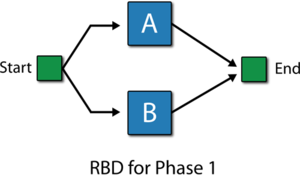
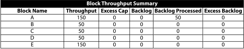
To examine throughput in phases, consider a phase diagram of three phases with linked RBDs, as shown in the figure below. Each phase has a duration of 10 hours and all phases are set to continue simulation upon failure. Blocks A through E process a number of items per hour as identified next to each letter (e.g., A:10 implies that 10 units are processed per hour by block A). Similarly, each phase is marked with the constant throughput sent to the blocks in the phase (e.g., P1:5 implies phase P1 sends 5 units to its blocks ). For the sake of simplicity, it is assumed that the blocks can never fail and that items are routed equally to each path (see Throughput Analysis Options). The ignore backlog option is left unchecked for all blocks in the phase diagram.
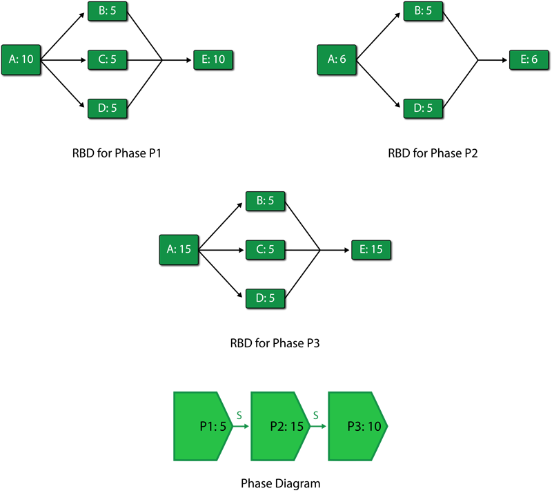
If the phase diagram is run on a throughput simulation with an end time of 60 hours, the following scenario can be observed:
- 1. Phase P1 from 0 to 10 hours
- a) Phase P1 sends 5 units in the first hour to block A. The capacity of block A in this phase is 10 units per hour. Block A processes these 5 units with an excess capacity of 5 units in the first hour.
- b) The 5 units processed by block A are routed equally over the three paths to blocks B, C and D. Each of these blocks receives 1.67 units in the first hour. The capacity of each of these blocks is 5 units per hour. Thus, blocks B, C and D each process 1.67 units with an excess capacity of 3.33 units in the first hour.
- c) Blocks B, C and D route each of their 1.67 units to E. The capacity of E in this phase is 10 units per hour. E processes the total of 5 units with an excess capacity of 5 units in the first hour.
- d) The above steps are repeated for the first ten hours to complete phase P1.
- 1. Phase P1 from 0 to 10 hours
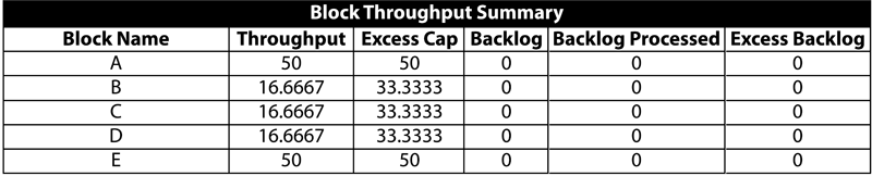
- A summary result table for phase P1 is shown next.
- 2. Phase P2 from 10 to 20 hours
- a) Phase P2 sends 15 units in its first hour to block A. The capacity of block A in this phase is changed from the previous phase and is now 6 units per hour. Thus, block A is able to process only 6 units while there is a backlog of 9 units per hour.
- b) The 6 units processed by block A are routed equally to blocks B and D as C is absent in this phase. Blocks B and D get 3 units each. The capacity of each of these blocks is 5 units per hour. Thus, blocks B and D process 3 units with an excess capacity of 2 units each in the first hour of the second phase.
- c) Blocks B and D route a total of 6 units to E. The capacity of block E in this phase is 6 units per hour. Thus, block E processes 6 units in the first hour of phase 2 with no excess capacity and no backlog.
- d) The above steps are repeated for the ten hours of phase P2. At 20 hours phase P2 ends.
- 2. Phase P2 from 10 to 20 hours
- A summary result table for phase P2 is shown next.

- 3. Phase P3 from 20 to 30 hours
- a) Phase P3 sends 10 units in its first hour to block A. The capacity of block A in this phase is now 15 units per hour. Thus, block A is able to process all 10 units sent by P3 and also process 5 units of the backlog from phase P2. Thus, during the first hour of phase P3, block A processes 15 units that includes a backlog of 5 units. Since block A is used to its full capacity, the excess capacity of A is zero.
- b) The 15 units processed by block A in the first hour are routed equally over three paths to blocks B, C and D as block C is available again in this phase. Blocks B, C and D receive 5 units each. The capacity of each of these block is 5 units per hour. Thus, blocks B, C and D process 5 units each to full capacity with no excess capacity during the first hour of the third phase.
- c) Blocks B, C and D route each of their 5 units to E. The capacity of block E in this phase is 15 units per hour. Thus, block E processes 15 units in the first hour of phase P3 with no excess capacity and no backlog.
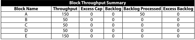
- d) The above steps are repeated for the ten hours of phase P3. It should be noted that although some of the backlog from phase P2 gets processed in phase P3 [math]\displaystyle{ (5\times 10=50\,\! }[/math] units from the backlog get processed ), not all 90 backlogged units are processed ( [math]\displaystyle{ 90-50 = 40\,\! }[/math] units remain). The remaining units cannot be shown as backlog for phase P3 because these were generated in phase P2. To avoid confusion between backlogs of different phases, BlockSim does not display backlog values at the individual phase levels. At 30 hours, phase P3 ends. This also ends the first cycle of the phase diagram.
- 3. Phase P3 from 20 to 30 hours
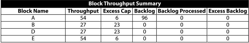
- A summary result table for phase P3 is shown next.
- A summary result table for phase P3 is shown next.
- 4. Phase P1 in the second cycle from 30 to 40 hours
- a) As in the first cycle, phase P1 sends 5 units to block A in the first hour. The capacity of block A in this phase is 10 units per hour. Thus, block A is able to process all 5 units sent by P1 and also process 5 units of the backlog from the first cycle. Thus, during the first hour of the second cycle of phase P1, block A processes 10 units that includes a backlog of 5 units. Since there is a backlog of 40 units from the first cycle, this is processed by block A in the first eight hours of the second cycle. During the last two hours of the second cycle of phase P1, block A processes only the 5 units per hour it receives from P1 and has an excess capacity of 5 units per hour. Thus, by the end of this phase, block A processes a total of 90 units (i.e., 50 units from P1 and 40 units of backlog) with an excess capacity of 10 units.
- b) Units processed by block A are routed equally to blocks B, C and D. During the first eight hours of the second cycle of phase P1, 10 units per hour are sent by block A to blocks B, C and D. Each of these blocks gets 3.33 units per hour. The capacity of each of these blocks is 5 units per hour. Thus, during the first eight hours of P1 in the second cycle, blocks B, C and D process 3.33 units per hour with an excess capacity of 1.67 units per hour. During the last two hours, block A processes 5 units per hour. Thus, blocks B, C and D process 1.67 units per hour with an excess capacity of 3.33 units per hour. At the end of the phase, blocks B, C and D each process a total of 30 units [math]\displaystyle{ (3.33\times 8+1.67\times 2=30)\,\! }[/math] with an excess capacity of 20 units [math]\displaystyle{ (1.67\times 8+3.33\times 2=20)\,\! }[/math].
- c) Blocks B, C and D route each of their units to block E. The capacity of E in this phase is 10 units per hour. Block E processes 10 units per hour with no excess capacity during the first eight hours of the phase. During the last two hours, block E processes 5 units per hour with an excess capacity of 5 units per hour. By the end of the phase, block E processes a total of 90 units with an excess capacity of 10 units.
- 4. Phase P1 in the second cycle from 30 to 40 hours
- A summary result table for the second cycle of phase P1 is shown next.
- 5. Phase P2 in the second cycle from 40 to 50 hours
- a) As in the first cycle, phase P2 sends 15 units in its first hour to block A. The capacity of block A in this phase is 6 units per hour. Thus, block A processes only 6 units while there is a backlog of 9 units per hour.
- b) The 6 units processed by block A are routed equally to blocks B and D, as C is absent in this phase. Blocks B and D receive 3 units each. The capacity of each of these blocks is 5 units per hour. Thus, in the second cycle, blocks B and D process 3 units each with an excess capacity of 2 units each in the first hour of the second phase.
- c) Blocks B and D route a total of 6 units to block E. The capacity of E in this phase is 6 units per hour. Thus, block E processes 6 units in the first hour of the phase with no excess capacity and no backlog.
- d) The above steps are repeated for the ten hours of phase P2. At 50 hours, phase P2 ends in the second cycle.
- 5. Phase P2 in the second cycle from 40 to 50 hours
- A summary result table for the second cycle of phase P2 is shown next.

- 6. Phase P3 in the second cycle from 50 to 60 hours
- a) Phase P3 sends 10 units in its first hour to block A in the second cycle. The capacity of block A in this phase is 15 units per hour. Thus, block A is able to process all 10 units sent by P3 and also process 5 units of backlog from the second cycle of phase P2. Thus, during the first hour of phase P3, block A processes 15 units that includes a backlog of 5 units. Since block A is used to its full capacity, the excess capacity of A is zero.
- b) The 15 units processed by block A in the first hour are routed equally over three paths to blocks B, C and D, as block C is available again in this phase. Blocks B, C and D receive 5 units each. The capacity of each of these block is 5 units per hour. Thus, blocks B, C and D process 5 units each to full capacity with no excess capacity during the first hour of the third phase.
- c) Blocks B, C and D route each of their 5 units to block E. The capacity of E in this phase is 15 units per hour. Thus, block E processes 15 units in the first hour of phase P3 with no excess capacity and no backlog.
- d) The above steps are repeated for the ten hours of phase P3. At 60 hours, phase P3 ends. This ends the second cycle of the phase diagram and also marks the end of the simulation.
- 6. Phase P3 in the second cycle from 50 to 60 hours
- A summary result table for the second cycle of phase P3 is shown next.
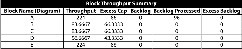
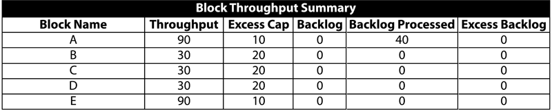
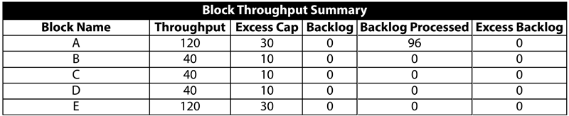
A summary result table for the overall system for the simulation from 0 to 60 hours is shown in the following table.
Variable (Time-Varying) Throughput
Time-varying throughput can be specified at the phase level through the Variable Throughput property of an operational phase. Variable throughput permits modeling of scenarios where the throughput changes over time. For variable throughput, three general models are available in BlockSim. Each of these models has two parameters a and b which are specified by the user. These models are discussed below:
- 1. Linear model:
- [math]\displaystyle{ \begin{align} y=ax+b \end{align}\,\! }[/math]
- This model describes the change in throughput [math]\displaystyle{ y\,\! }[/math] as a linear function of time [math]\displaystyle{ x\,\! }[/math]. Throughput processed between any two points of time [math]\displaystyle{ {{x}}_{{1}}\,\! }[/math] and [math]\displaystyle{ {{x}}_{{2}}\,\! }[/math] is obtained by integration of the linear function as:
- [math]\displaystyle{ \begin{align} \text{Linearly varying throughput}= & \mathop{}_{{{x}_{1}}}^{{{x}_{2}}}ydx \\ = & \mathop{}_{{{x}_{1}}}^{{{x}_{2}}}(ax+b)dx \\ = & \frac{a}{2}(x_{2}^{2}-x_{1}^{2})+b({{x}_{2}}-{{x}_{1}}) \end{align}\,\! }[/math]
- 2. Exponential model:
- [math]\displaystyle{ \begin{align} y={be}^{ax} \end{align}\,\! }[/math]
- This model describes the change in throughput [math]\displaystyle{ y\,\! }[/math] as an exponential function of time [math]\displaystyle{ x\,\! }[/math]. Throughput processed in a period of time between any two points [math]\displaystyle{ {{x}}_{{1}}\,\! }[/math] and [math]\displaystyle{ {{x}}_{{2}}\,\! }[/math] is obtained as:
- [math]\displaystyle{ \begin{align} \text{Exponentially varying throughput}= & \mathop{}_{{{x}_{1}}}^{{{x}_{2}}}ydx \\ = & \mathop{}_{{{x}_{1}}}^{{{x}_{2}}}b{{e}^{ax}}dx \\ = & \text{ }\frac{b}{a}({{e}^{a{{x}_{2}}}}-{{e}^{a{{x}_{1}}}}) \end{align}\,\! }[/math]
- 3. Power model:
- [math]\displaystyle{ \begin{align} y={bx}^{a} \end{align}\,\! }[/math]
- This model describes the change in throughput [math]\displaystyle{ y\,\! }[/math] as a power function of time [math]\displaystyle{ x\,\! }[/math]. Throughput processed between two points of time [math]\displaystyle{ {{x}}_{{1}}\,\! }[/math] and [math]\displaystyle{ {{x}}_{{2}}\,\! }[/math] is obtained as:
- [math]\displaystyle{ \begin{align} \text{Power varying throughput}= & \mathop{}_{{{x}_{1}}}^{{{x}_{2}}}ydx \\ = & \mathop{}_{{{x}_{1}}}^{{{x}_{2}}}b{{x}^{a}}dx \\ = & \frac{b}{a+1}(x_{2}^{a+1}-x_{1}^{a+1}) \end{align}\,\! }[/math]
All of the above models also have a user defined maximum throughput capacity value. Once this maximum throughput capacity value is reached, the throughput per unit time becomes constant and equal in value to the maximum throughput capacity specified by the user. In this situation, the variable throughput model would then act as a constant throughput model. The above models may at first glance seem limited, when in fact they do provide ample modeling flexibility. This flexibility is achieved by using these functions as building blocks for more complex functions. As an example, a step model can be easily created by using multiple phases, each with a constant throughput. A ramp model would use phases with linearly increasing functions in conjunction with constant phases, and so forth.
Variable Throughput Example
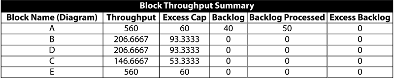
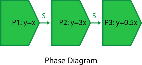
To examine variable throughput in phase diagrams, consider the phase diagram used above in the constant throughput example. All phase properties and linked RBDs remain unchanged for this illustration except that all the three phases now use variable throughput models. For the first phase, P1, the variable throughput model used is [math]\displaystyle{ y = x\,\! }[/math] (which is the linear model [math]\displaystyle{ y = ax+ b\,\! }[/math] with parameters [math]\displaystyle{ a = 1\,\! }[/math] and [math]\displaystyle{ b = 0\,\! }[/math]). For the second phase, P2, the model used is [math]\displaystyle{ y = 3x\,\! }[/math] (which is the linear model [math]\displaystyle{ y = ax+ b\,\! }[/math] with parameters [math]\displaystyle{ a = 3\,\! }[/math] and [math]\displaystyle{ b = 0\,\! }[/math]). The third phase uses [math]\displaystyle{ y = 0.5x\,\! }[/math] as the variable throughput model (which is the linear model [math]\displaystyle{ y = ax + b\,\! }[/math] with parameters [math]\displaystyle{ a = 0.5\,\! }[/math] and [math]\displaystyle{ b = 0\,\! }[/math]). Phases P1 and P2 have a value of 500 units per hour set for the maximum throughput capacity. This relatively larger value of throughput is set for the two phases so that the phases do not reach their maximum throughput value during the simulation. Phase P3 has a value of 4 units per hour set as the maximum throughput capacity. As in the previous example, all phases have a duration of ten hours. For the sake of simplicity it is assumed that the blocks can never fail and that items are routed equally to each path. The ignore backlog option is left unchecked for all blocks in the phase diagram.
If a throughput simulation with an end time of 60 hours is run on the phase diagram, the following scenario can be observed:
- 1. Phase P1 from 0 to 10 hours
- a) The throughput from phase P1 follows a time-varying model given by [math]\displaystyle{ y = ax + b\,\! }[/math] with parameters [math]\displaystyle{ a = 1\,\! }[/math] and [math]\displaystyle{ b = 0\,\! }[/math]. Thus, during the first hour the throughput sent by phase P1 to block A is:
- [math]\displaystyle{ \begin{align} Phase throughput from 0 to 1hr= & \frac{a}{2}(x_{2}^{2}-x_{1}^{2})+b({{x}_{2}}-{{x}_{1}}) \\ = & \frac{1}{2}({{1}^{2}}-{{0}^{2}})+0(1-0) \\ = & 0.5\text{ }units \end{align}\,\! }[/math]
- And the throughput sent by phase P1 to block A in the second hour is:
- [math]\displaystyle{ \begin{align} Phase throughput from 1 to 2 hrs= & \frac{a}{2}(x_{2}^{2}-x_{1}^{2})+b({{x}_{2}}-{{x}_{1}}) \\ = & \frac{1}{2}({{2}^{2}}-{{1}^{2}})+0(2-1) \\ = & 1.5\text{ }units \end{align}\,\! }[/math]
- It can be seen that the throughput from phase P1 sent to block A increases with time. But the capacity of block A remains constant at 10 units per hour during the entire phase P1. Thus, it becomes important to know the point of time when the number of units sent by P1 exceed the capacity of block A and the block starts accumulating a backlog. This can be obtained by solving the throughput model for phase P1 [math]\displaystyle{ (y = x)\,\! }[/math] using the capacity of block A by substituting [math]\displaystyle{ y\,\! }[/math] as the block capacity as shown next:
- [math]\displaystyle{ \begin{align} y= & x \\ or\text{ }10= & x \end{align}\,\! }[/math]
- Thus, at time [math]\displaystyle{ x = 10\,\! }[/math] hours the number of units supplied per hour by phase P1 will equal the capacity of block A. At this point of time block A will function to its full capacity with no excess capacity and no backlog. Beyond this point the units sent by phase P1 will exceed the capacity of block A and the block will start accumulating a backlog. Since the duration of phase P1 is 10 hours, backlog at block A will not be a concern in this phase because up to this time the capacity of the block exceeds the units sent by phase P1. Thus, the total units sent by phase P1 to block A during the phase duration of 10 hours is:
- [math]\displaystyle{ \begin{align} = & \frac{a}{2}(x_{2}^{2}-x_{1}^{2})+b({{x}_{2}}-{{x}_{1}}) \\ = & \frac{1}{2}({{10}^{2}}-{{0}^{2}})+0(10-0) \\ = & 50\text{ }units \end{align}\,\! }[/math]
- The total number of units that can be processed by block A (or the capacity of A) during phase P1 is:
- [math]\displaystyle{ \begin{align} = & 10\times 10 \\ = & 100\text{ }units \end{align}\,\! }[/math]
- Thus, during the first phase, block A processes all 50 units sent by phase P1 with an excess capacity of 50 units (100-50=50 units).
- b) The 50 units processed by block A from time 0 to 10 hours are routed equally over three paths to blocks B, C and D. Each of these blocks gets a total of 16.67 units from time 0 to 10 hours. The capacity of each of these blocks is 5 units per hour. Thus, the total capacity of each of the blocks from time 0 to 10 hours is 50 units. As a result, each of the three blocks processes 16.67 units in phase P1 with an excess capacity of 33.33 units.
- c) Blocks B, C and D route each of their 16.67 units to block E. The capacity of E in this phase is 10 units per hour or 100 units for the ten hours. Thus, block E processes a total of 50 units from blocks B, C and D with an excess capacity of 50 units during the first phase P1. At 10 hours, phase P1 ends and phase P2 begins.
- A summary result table for phase P1 is shown next.
- 2. Phase P2 from 10 to 20 hours
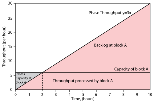
- a) The throughput of phase P2 follows the model [math]\displaystyle{ y = ax + b\,\! }[/math] with [math]\displaystyle{ a = 3\,\! }[/math] and [math]\displaystyle{ b = 0\,\! }[/math]. The throughput from P2 goes to block A. The capacity of block A in this phase is 6 units per hour. The point of time when the number of units sent by P2 equals the capacity of block A can be obtained by substituting the capacity of block A into the model equation [math]\displaystyle{ (y = 3x)\,\! }[/math] as shown next:
- [math]\displaystyle{ \begin{align} y= & 3x \\ or\text{ }6= & 3x \\ or\text{ }x= & 2 \end{align}\,\! }[/math]
- Thus, at [math]\displaystyle{ x = 2\,\! }[/math] hours of phase P2 (or at the total simulation time of 12 hours), the number of units sent per hour by phase P2 equals the capacity of block A. Thus, during the first two hours of phase P2, block A will have excess capacity. The total number of units sent by phase P2 during the first two hours of the phase is:
- [math]\displaystyle{ \begin{align} = & \frac{a}{2}(x_{2}^{2}-x_{1}^{2})+b({{x}_{2}}-{{x}_{1}}) \\ = & \frac{3}{2}({{2}^{2}}-{{0}^{2}})+0(2-0) \\ = & 6\text{ }units \end{align}\,\! }[/math]
- The total capacity of block A during the first two hours of phase P2 is:
- [math]\displaystyle{ \begin{align} = & 6\times 2 \\ = & 12\text{ }units \end{align}\,\! }[/math]
- Thus block A processes a total of 6 units in the first two hours of phase P2 with an excess capacity of 6 units (12-6=6 units). During the last eight hours of the phase (from the second hour to the tenth hour) block A will have a backlog because the number of units sent by phase P2 will exceed block A's capacity. The total number of units sent by phase P2 during the last eight hours of the phase is:
- [math]\displaystyle{ \begin{align} = & \frac{a}{2}(x_{2}^{2}-x_{1}^{2})+b({{x}_{2}}-{{x}_{1}}) \\ = & \frac{3}{2}({{10}^{2}}-{{2}^{2}})+0(10-2) \\ = & 144\text{ }units \end{align}\,\! }[/math]
- The total capacity of block A during these eight hours of phase P2 is:
- [math]\displaystyle{ \begin{align} = & 6\times 8 \\ = & 48\text{ }units \end{align}\,\! }[/math]
- Thus, during the last eight hours of phase P2, block A will process a total of 48 units with a backlog of 96 units (144-48=96 units). A graphical representation of the above scenario for block A during phase P2 is shown in the figure below.
- b) The units processed by block A are routed equally to blocks B and D, as block C is absent in this phase. During the first two hours, block A sends a total of 6 units that are divided equally among blocks B and D, with each block getting 3 units. The capacity of these blocks in this phase is 5 units per hour. Thus the total capacity of each of these blocks during the first two hours of phase P2 is:
- [math]\displaystyle{ \begin{align} = & 5\times 2 \\ = & 10\text{ }units \end{align}\,\! }[/math]
- As a result, blocks B and D each process 3 units in the first two hours of phase P2 with an excess capacity of 7 units (10-3=7 units). During the last eight hours of phase P2, block A sends a total of 48 units to blocks B and D, with each block receiving 24 units. The capacity of each of these blocks during these eight hours is:
- [math]\displaystyle{ \begin{align} = & 5\times 8 \\ = & 40\text{ }units \end{align}\,\! }[/math]
- Thus, B and D process 24 units in the last eight hours of phase P2, with an excess capacity of 16 units (40-24=16 units).
- c) The units processed by blocks B and D are sent to block E. The capacity of E in this phase is 6 units per hour. During the first two hours of phase P2, a total of 6 units are sent to block E. The total capacity of block E during this period of time is:
- [math]\displaystyle{ \begin{align} = & 6\times 2 \\ = & 12\text{ }units \end{align}\,\! }[/math]
- Consequently block E processes 6 units in the first two hours of phase P2 with an excess capacity of 6 units (12-6=6 units). During the last eight hours of the phase, blocks B and D send a total of 48 units to block E. The capacity of block E during this time is:
- [math]\displaystyle{ \begin{align} = & 6\times 8 \\ = & 48\text{ }units \end{align}\,\! }[/math]
- Thus, block E processes 48 units in the last eight hours of P2 with no excess capacity and no backlog. At 20 hrs phase P2 ends and phase P3 begins.
- A summary result table for phase P2 is shown next.
- 3. Phase P3 from 20 to 30 hours
- a) The throughput of phase P3 follows the model [math]\displaystyle{ y = ax + b\,\! }[/math] with [math]\displaystyle{ a = 0.5\,\! }[/math] and [math]\displaystyle{ b = 0\,\! }[/math]. A maximum throughput capacity of 4 units per hour is also set for this phase. The throughput from this phase goes to block A. The capacity of block A in this phase is 15 units per hour. Thus, it can be seen that the throughput sent by phase P3 will never exceed the capacity of block A in this phase. It can also be seen that at some point of time the throughput of phase P3 will reach the maximum throughput capacity of 4 units per hour and, thereafter, a constant throughput of 4 units per hour will be sent by phase P3. This point of time can be calculated by solving the linear throughput model for the phase [math]\displaystyle{ y = 0.5x\,\! }[/math] by substituting [math]\displaystyle{ y\,\! }[/math] as the maximum throughput capacity as shown next:
- [math]\displaystyle{ \begin{align} y= & 0.5x \\ or\text{ }4= & 0.5x \\ or\text{ }x= & 8 \end{align}\,\! }[/math]
- Thus, at time [math]\displaystyle{ x = 8\,\! }[/math] hours of phase P3 (or at the time of 28 hours) the number of units sent per hour by phase P3 will reach the constant value of 4 units per hour. In the first eight hours of the phase the throughput will remain variable. The total number of units sent by P3 to block A during this time is given by:
- [math]\displaystyle{ \begin{align} = & \frac{a}{2}(x_{2}^{2}-x_{1}^{2})+b({{x}_{2}}-{{x}_{1}}) \\ = & \frac{0.5}{2}({{8}^{2}}-{{0}^{2}})+0(8-0) \\ = & 16\text{ }units \end{align}\,\! }[/math]
- The total capacity of block A during the first eight hours of phase P3 is:
- [math]\displaystyle{ \begin{align} = & 15\times 8 \\ = & 120\text{ }units \end{align}\,\! }[/math]
- Consequently, it can be seen that block A has an excess capacity of 104 units (120-16=104 units). Thus, block A will be able to process all of the 96 units of backlog from phase P2 during these eight hours. As a result, block A will process a total of 112 units (16 units from P3 and 96 units from the backlog of phase P2) with an excess capacity of 8 units (120-112=8 units) during the first eight hours of phase P3. In the last two hours of this phase, a constant throughput of 4 units per hour is sent to block A, thus the total number of units sent to the block during the last two hours are:
- [math]\displaystyle{ \begin{align} = & 4\times 2 \\ = & 8\text{ }units \end{align}\,\! }[/math]
- The capacity of block A during these two hours is:
- [math]\displaystyle{ \begin{align} = & 15\times 2 \\ = & 30\text{ }units \end{align}\,\! }[/math]
- Thus, block A will process 8 units in the last two hours of phase P3 with an excess capacity of 22 units (30-8=22 units).
- b) The units processed by block A are routed equally over three paths to blocks B, C and D, as block C is available again in this phase. During the first eight hours of phase P3 a total of 112 units are sent to blocks B, C and D, with each block receiving 37.33 units. The capacity of each of these block is 5 units per hour, thus the total capacity of each of the blocks during the first eight hours is:
- [math]\displaystyle{ \begin{align} = & 5\times 8 \\ = & 40\text{ }units \end{align}\,\! }[/math]
- As a result, blocks B, C and D each process 37.33 units in the first eight hour of phase P3 with an excess capacity of 2.67 units (40-37.33=2.67 units). In the last two hours of the phase, block A sends a total of 8 units, with each block getting 2.67 units. The capacity of blocks B, C or D during these two hours is:
- [math]\displaystyle{ \begin{align} = & 5\times 2 \\ = & 10\text{ }units \end{align}\,\! }[/math]
- Thus, blocks B, C and D each process 2.67 units in the last two hours of phase P3 with an excess capacity of 7.33 units (10-2.67=7.33 units). At the end of these two hours phase P3 gets completed. This also marks the end of the simulation.
- A summary result table for phase P3 is shown next.
A summary result table for the overall system for the simulation from 0 to 30 hrs is shown in the following table.