Repairable Systems Analysis Through Simulation

Having introduced some of the basic theory and terminology for repairable systems in Chapter 7, we will now examine the steps involved in the analysis of such complex systems. We will begin by examining system behavior through a sequence of discrete deterministic events and expand the analysis using discrete event simulation.

Simple Repairs

Deterministic View, Simple Series

To first understand how component failures and simple repairs affect the system and to visualize the steps involved, let's begin with a very simple deterministic example with two components, [math]\displaystyle{ A }[/math] and [math]\displaystyle{ B }[/math], in series.

Component [math]\displaystyle{ A }[/math] fails every 100 hours and component [math]\displaystyle{ B }[/math] fails every 120 hours. Both require 10 hours to get repaired. Furthermore, assume that the surviving component stops operating when the system fails (thus not aging). NOTE: When a failure occurs in certain systems, some or all of the system's components may or may not continue to accumulate operating time while the system is down. For example, consider a transmitter-satellite-receiver system. This is a series system and the probability of failure for this system is the probability that any of the subsystems fail. If the receiver fails, the satellite continues to operate even though the receiver is down. In this case, the continued aging of the components during the system inoperation must be taken into consideration, since this will affect their failure characteristics and have an impact on the overall system downtime and availability.
The system behavior during an operation from 0 to 300 hours would be as shown in figure below.

Specifically, component [math]\displaystyle{ A }[/math] would fail at 100 hours, causing the system to fail. After 10 hours, component [math]\displaystyle{ A }[/math] would be restored and so would the system. The next event would be the failure of component [math]\displaystyle{ B }[/math] . We know that component [math]\displaystyle{ B }[/math] fails every 120 hours (or after an age of 120 hours). Since a component does not age while the system is down, component [math]\displaystyle{ B }[/math] would have reached an age of 120 when the clock reaches 130 hours. Thus, component [math]\displaystyle{ B }[/math] would fail at 130 hours and be repaired by 140 and so forth. Overall in this scenario, the system would be failed for a total of 40 hours due to four downing events (two due to [math]\displaystyle{ A }[/math] and two due to [math]\displaystyle{ B }[/math] ). The overall system availability (average or mean availability) would be [math]\displaystyle{ 260/300=0.86667 }[/math] . Point availability is the availability at a specific point time. In this deterministic case, the point availability would always be equal to 1 if the system is up at that time and equal to zero if the system is down at that time.

Operating Through System Failure

In the prior section we made the assumption that components do not age when the system is down. This assumption applies to most systems. However, under special circumstances, a unit may age even while the system is down. In such cases, the operating profile will be different from the one presented in the prior section. Figure below illustrates the case where the components operate continuously, regardless of the system status.

Effects of Operating Through Failure

Consider a component with an increasing failure rate, as shown in figure below. In the case that the component continues to operate through system failure, then when the system fails at [math]\displaystyle{ {{t}_{1}} }[/math] the surviving component's failure rate will be [math]\displaystyle{ {{\lambda }_{1}} }[/math] , as illustrated in figure below. When the system is restored at [math]\displaystyle{ {{t}_{2}} }[/math] , the component would have aged by [math]\displaystyle{ {{t}_{2}}-{{t}_{1}} }[/math] and its failure rate would now be [math]\displaystyle{ {{\lambda }_{2}} }[/math] .

In the case of a component that does not operate through failure, then the surviving component would be at the same failure rate, [math]\displaystyle{ {{\lambda }_{1}}, }[/math] when the system resumes operation.

Deterministic View, Simple Parallel

Consider the following system where [math]\displaystyle{ A }[/math] fails every 100, [math]\displaystyle{ B }[/math] every 120, [math]\displaystyle{ C }[/math] every 140 and [math]\displaystyle{ D }[/math] every 160 time units. Each takes 10 time units to restore. Furthermore, assume that components do not age when the system is down.

A deterministic system view is shown in Figure "Overview of simple redundant system with four components". The sequence of events is as follows:

1. At 100, [math]\displaystyle{ A }[/math] fails and is repaired by 110. The system is failed.
2. At 130, [math]\displaystyle{ B }[/math] fails and is repaired by 140. The system continues to operate.
3. At 150, [math]\displaystyle{ C }[/math] fails and is repaired by 160. The system continues to operate.
4. At 170, [math]\displaystyle{ D }[/math] fails and is repaired by 180. The system is failed.
5. At 220, [math]\displaystyle{ A }[/math] fails and is repaired by 230. The system is failed.
6. At 280, [math]\displaystyle{ B }[/math] fails and is repaired by 290. The system continues to operate.
7. End at 300.

Additional Notes

It should be noted that we are dealing with these events deterministically in order to better illustrate the methodology. When dealing with deterministic events, it is possible to create a sequence of events that one would not expect to encounter probabilistically. One such example consists of two units in series that do not operate through failure but both fail at exactly 100, which is highly unlikely in a real-world scenario. In this case, the assumption is that one of the events must occur at least an infinitesimal amount of time ( [math]\displaystyle{ dt) }[/math] before the other. Probabilistically, this event is extremely rare, since both randomly generated times would have to be exactly equal to each other, to 15 decimal points. In the rare event that this happens, BlockSim would pick the unit with the lowest ID value as the first failure. BlockSim assigns a unique numerical ID when each component is created. These can be viewed by selecting the Show Block ID option in the Diagram Options window.

Deterministic Views of More Complex Systems

Even though the examples presented are fairly simplistic, the same approach can be repeated for larger and more complex systems. The reader can easily observe/visualize the behavior of more complex systems in BlockSim using the Up/Down plots. These are the same plots used in this chapter. It should be noted that BlockSim makes these plots available only when a single simulation run has been performed for the analysis (i.e. Number of Simulations = 1). These plots are meaningless when doing multiple simulations because each run will yield a different plot.

Probabilistic View, Simple Series

In a probabilistic case, the failures and repairs do not happen at a fixed time and for a fixed duration, but rather occur randomly and based on an underlying distribution, as shown in Figures "A single component with a probabilistic failure time and repair duration" and Figure "A system up/down plot illustrating a probabilistic failure time and repair duration for component B".

We use discrete event simulation in order to analyze (understand) the system behavior. Discrete event simulation looks at each system/component event very similarly to the way we looked at these events in the deterministic example. However, instead of using deterministic (fixed) times for each event occurrence or duration, random times are used. These random times are obtained from the underlying distribution for each event. As an example, consider an event following a 2-parameter Weibull distribution. The [math]\displaystyle{ cdf }[/math] of the 2-parameter Weibull distribution is given by:

[math]\displaystyle{ F(T)=1-{{e}^{-{{\left( \tfrac{T}{\eta } \right)}^{\beta }}}} }[/math]

The Weibull reliability function is given by:

[math]\displaystyle{ \begin{align} R(T)= & 1-F(t) \\ = & {{e}^{-{{\left( \tfrac{T}{\eta } \right)}^{\beta }}}} \end{align} }[/math]

Then, to generate a random time from a Weibull distribution with a given [math]\displaystyle{ \eta }[/math] and [math]\displaystyle{ \beta }[/math] , a uniform random number from 0 to 1, [math]\displaystyle{ {{U}_{R}}[0,1] }[/math] , is first obtained. The random time from a Weibull distribution is then obtained from:

[math]\displaystyle{ {{T}_{R}}=\eta \cdot {{\left\{ -\ln \left[ {{U}_{R}}[0,1] \right] \right\}}^{\tfrac{1}{\beta }}}(eqn 1) }[/math]

To obtain a conditional time, the Weibull conditional reliability function is given by:

[math]\displaystyle{ R(T,t)=\frac{R(T+t)}{R(T)}=\frac{{{e}^{-{{\left( \tfrac{T+t}{\eta } \right)}^{\beta }}}}}{{{e}^{-{{\left( \tfrac{T}{\eta } \right)}^{\beta }}}}}(eqn 2) }[/math]

Or:

[math]\displaystyle{ R(T,t)={{e}^{-\left[ {{\left( \tfrac{T+t}{\eta } \right)}^{\beta }}-{{\left( \tfrac{T}{\eta } \right)}^{\beta }} \right]}} }[/math]

The random time would be the solution for [math]\displaystyle{ t }[/math] for [math]\displaystyle{ R(T,t)={{U}_{R}}[0,1] }[/math] .
To illustrate the sequence of events, assume a single block with a failure and a repair distribution. The first event, [math]\displaystyle{ {{E}_{{{F}_{1}}}} }[/math] , would be the failure of the component. Its first time-to-failure would be a random number drawn from its failure distribution, [math]\displaystyle{ {{T}_{{{F}_{1}}}} }[/math] . Thus, the first failure event, [math]\displaystyle{ {{E}_{{{F}_{1}}}} }[/math] , would be at [math]\displaystyle{ {{T}_{{{F}_{1}}}} }[/math] . Once failed, the next event would be the repair of the component, [math]\displaystyle{ {{E}_{{{R}_{1}}}} }[/math] . The time to repair the component would now be drawn from its repair distribution, [math]\displaystyle{ {{T}_{{{R}_{1}}}} }[/math] . The component would be restored by time [math]\displaystyle{ {{T}_{{{F}_{1}}}}+{{T}_{{{R}_{1}}}} }[/math] . The next event would now be the second failure of the component after the repair, [math]\displaystyle{ {{E}_{{{F}_{2}}}} }[/math] . This event would occur after a component operating time of [math]\displaystyle{ {{T}_{{{F}_{2}}}} }[/math] after the item is restored (again drawn from the failure distribution), or at [math]\displaystyle{ {{T}_{{{F}_{1}}}}+{{T}_{{{R}_{1}}}}+{{T}_{{{F}_{2}}}} }[/math] . This process is repeated until the end time. It is important to note that each run will yield a different sequence of events due to the probabilistic nature of the times. To arrive at the desired result, this process is repeated many times and the results from each run (simulation) are recorded. In other words, if we were to repeat this 1,000 times, we would obtain 1,000 different values for [math]\displaystyle{ {{E}_{{{F}_{1}}}} }[/math] , or [math]\displaystyle{ \left[ {{E}_{{{F}_{{{1}_{1}}}}}},{{E}_{{{F}_{{{1}_{2}}}}}},...,{{E}_{{{F}_{{{1}_{1,000}}}}}} \right] }[/math].

The average of these values, [math]\displaystyle{ \left( \tfrac{1}{1000}\underset{i=1}{\overset{1,000}{\mathop{\sum }}}\,{{E}_{{{F}_{{{1}_{i}}}}}} \right) }[/math] , would then be the average time to the first event, [math]\displaystyle{ {{E}_{{{F}_{1}}}} }[/math] , or the mean time to first failure (MTTFF) for the component. Obviously, if the component were to be 100% renewed after each repair, then this value would also be the same for the second failure, etc.

General Simulation Results

To further illustrate this, assume that components A and B in the prior example had normal failure and repair distributions with their means equal to the deterministic values used in the prior example and standard deviations of 10 and 1 respectively. That is, [math]\displaystyle{ {{F}_{A}}\tilde{\ }N(100,10), }[/math] [math]\displaystyle{ {{F}_{B}}\tilde{\ }N(120,10), }[/math] [math]\displaystyle{ {{R}_{A}}={{R}_{B}}\tilde{\ }N(10,1) }[/math] . The settings for components C and D are not changed. Obviously, given the probabilistic nature of the example, the times to each event will vary. If one were to repeat this [math]\displaystyle{ X }[/math] number of times, one would arrive at the results of interest for the system and its components. Some of the results for this system and this example, over 1,000 simulations, are given in Figure "Summary of system results for 1,000 simulations" and explained in the next sections. The simulation settings are shown in figure below.

General

Std Deviation (Mean Availability)

This is the standard deviation of the mean availability of all downing events for the system during the simulation.

Mean Availability (w/o PM, OC & Inspection), [math]\displaystyle{ {{\overline{A}}_{CM}} }[/math]

This is the mean availability due to failure events only and it is 0.971 for this example. Note that for this case, the mean availability without preventive maintenance, on condition maintenance and inspection is identical to the mean availability for all events. This is because no preventive maintenance actions or inspections were defined for this system. We will discuss the inclusion of these actions in later sections.

Downtimes caused by PM and inspections are not included. However, if the PM or inspection action results in the discovery of a failure, then these times are included. As an example, consider a component that has failed but its failure is not discovered until the component is inspected. Then the downtime from the time failed to the time restored after the inspection is counted as failure downtime, since the original event that caused this was the component's failure.

Expected Number of Failures, [math]\displaystyle{ {{N}_{F}} }[/math]

This is the average number of system failures. The system failures (not downing events) for all simulations are counted and then averaged. For this case, this is 3.188, which implies that a total of 3,188 system failure events occurred over 1000 simulations. Thus, the expected number of system failures for one run is 3.188. This number includes all failures, even those that may have a duration of zero.

Std Deviation (Number of Failures)

This is the standard deviation of the number of failures for the system during the simulation.

MTTFF

MTTFF is the mean time to first failure for the system. This is computed by keeping track of the time at which the first system failure occurred for each simulation. MTTFF is then the average of these times. This may or may not be identical to the MTTF obtained in the analytical solution for the same reasons as those discussed in the Point Reliability section. For this case, this is 100.2511. This is fairly obvious for this case since the mean of one of the components in series was 100 hours.

It is important to note that for each simulation run, if a first failure time is observed, then this is recorded as the system time to first failure. If no failure is observed in the system, then the simulation end time is used as a right censored (suspended) data point. MTTFF is then computed using the total operating time until the first failure divided by the number of observed failures (constant failure rate assumption). Furthermore, and if the simulation end time is much less than the time to first failure for the system, it is also possible that all data points are right censored (i.e. no system failures were observed). In this case, the MTTFF is again computed using a constant failure rate assumption, or:

[math]\displaystyle{ MTTFF=\frac{2\cdot ({{T}_{S}})\cdot N}{\chi _{0.50;2}^{2}} }[/math]

Where [math]\displaystyle{ {{T}_{S}} }[/math] is the simulation end time and [math]\displaystyle{ N }[/math] is the number of simulations. One should be aware that this formulation may yield unrealistic (or erroneous) results if the system does not have a constant failure rate. If you are trying to obtain an accurate (realistic) estimate of this value, then your simulation end time should be set to a value that is well beyond the MTTF of the system (as computed analytically). As a general rule, the simulation end time should be at least three times larger than the MTTF of the system.

System Downing Events

System downing events are events associated with downtime. Note that events with zero duration will appear in this section only if the task properties specify that the task brings the system down or if the task properties specify that the task brings the item down and the item’s failure brings the system down.

Number of Failures, [math]\displaystyle{ {{N}_{{{F}_{Down}}}} }[/math]

This is the average number of system downing failures. Unlike the Expected Number of Failures, [math]\displaystyle{ {{N}_{F}}, }[/math] this number does not include failures with zero duration. For this example, this is 3.188.

Number of CMs, [math]\displaystyle{ {{N}_{C{{M}_{Down}}}} }[/math]

This is the number of corrective maintenance actions that caused the system to fail. It is obtained by taking the sum of all CM actions that caused the system to fail divided by the number of simulations. It does not include CM events of zero duration. For this example, this is 3.188. Note that this may differ from the Number of Failures, [math]\displaystyle{ {{N}_{{{F}_{Down}}}} }[/math] . An example would be a case where the system has failed, but due to other settings for the simulation, a CM is not initiated (e.g. an inspection is needed to initiate a CM).

Number of Inspections, [math]\displaystyle{ {{N}_{{{I}_{Down}}}} }[/math]

This is the number of inspection actions that caused the system to fail. It is obtained by taking the sum of all inspection actions that caused the system to fail divided by the number of simulations. It does not include inspection events of zero duration. For this example, this is zero.

Number of PMs, [math]\displaystyle{ {{N}_{P{{M}_{Down}}}} }[/math]

This is the number of PM actions that caused the system to fail. It is obtained by taking the sum of all PM actions that caused the system to fail divided by the number of simulations. It does not include PM events of zero duration. For this example, this is zero.

Number of OCs, [math]\displaystyle{ {{N}_{O{{C}_{Down}}}} }[/math]

This is the number of OC actions that caused the system to fail. It is obtained by taking the sum of all OC actions that caused the system to fail divided by the number of simulations. It does not include OC events of zero duration. For this example, this is zero.

Total Events, [math]\displaystyle{ {{N}_{AL{{L}_{Down}}}} }[/math]

This is the total number of system downing events. It also does not include events of zero duration. It is possible that this number may differ from the sum of the other listed events. As an example, consider the case where a failure does not get repaired until an inspection, but the inspection occurs after the simulation end time. In this case, the number of inspections, CMs and PMs will be zero while the number of total events will be one.

Costs and Throughput

Cost and throughput results are discussed in later sections.

Note About Overlapping Downing Events

It is important to note that two identical system downing events (that are continuous or overlapping) may be counted and viewed differently. As shown in Case 1 of figure below, two overlapping failure events are counted as only one event from the system perspective because the system was never restored and remained in the same down state, even though that state was caused by two different components. Thus, the number of downing events in this case is one and the duration is as shown in CM system. In the case that the events are different, as shown in Case 2 of figure below, two events are counted, the CM and the PM. However, the downtime attributed to each event is different from the actual time of each event. In this case, the system was first down due to a CM and remained in a down state due to the CM until that action was over. However, immediately upon completion of that action, the system remained down but now due to a PM action. In this case, only the PM action portion that kept the system down is counted.

System Point Result

The system point results, as shown in figure below, shows the Point Availability (All Events), [math]\displaystyle{ A\left( t \right) }[/math] , and Point Reliability, [math]\displaystyle{ R(t) }[/math] , as defined in the previous section. These are computed and returned at different points in time, based on the number of intervals selected by the user. Additionally, this window shows [math]\displaystyle{ (1-A(t)) }[/math] , [math]\displaystyle{ (1-R(t)) }[/math] , [math]\displaystyle{ \text{Labor Cost(t)} }[/math] ,[math]\displaystyle{ \text{Part Cost(t)} }[/math] , [math]\displaystyle{ Cost(t) }[/math] , [math]\displaystyle{ Mean }[/math] [math]\displaystyle{ A(t) }[/math] , [math]\displaystyle{ Mean }[/math] [math]\displaystyle{ A({{t}_{i}}-{{t}_{i-1}}) }[/math] , [math]\displaystyle{ System }[/math], [math]\displaystyle{ Failures(t) }[/math], [math]\displaystyle{ \text{System Off Events by Trigger(t)} }[/math] and [math]\displaystyle{ Throughput(t) }[/math] .

Results by Component

Simulation results for each component can also be viewed. Figure below shows the results for component A. These results are explained in the sections that follow.

General Information

Number of Block Downing Events, [math]\displaystyle{ Componen{{t}_{NDE}} }[/math]

This the number of times the component went down (failed). It includes all downing events.

Number of System Downing Events, [math]\displaystyle{ Componen{{t}_{NSDE}} }[/math]

This is the number of times that this component's downing caused the system to be down. For component [math]\displaystyle{ A }[/math] , this is 2.038. Note that this value is the same in this case as the number of component failures, since the component A is reliability-wise in series with components D and components B, C. If this were not the case (e.g. if they were in a parallel configuration, like B and C), this value would be different.

Number of Failures, [math]\displaystyle{ Componen{{t}_{NF}} }[/math]

This is the number of times the component failed and does not include other downing events. Note that this could also be interpreted as the number of spare parts required for CM actions for this component. For component [math]\displaystyle{ A }[/math] , this is 2.038.

Number of System Downing Failures, [math]\displaystyle{ Componen{{t}_{NSDF}} }[/math]

This is the number of times that this component's failure caused the system to be down. Note that this may be different from the Number of System Downing Events. It only counts the failure events that downed the system and does not include zero duration system failures.

Number of OFF events by Trigger, [math]\displaystyle{ Componen{{t}_{OFF}} }[/math]

The total number of events where the block is turned off by state change triggers. An OFF event is not a failure but it may be included in system reliability calculations.

Mean Availability (All Events), [math]\displaystyle{ {{\overline{A}}_{AL{{L}_{Component}}}} }[/math]

This has the same definition as for the system with the exception that this accounts only for the component.

Mean Availability (w/o PM, OC & Inspection), [math]\displaystyle{ {{\overline{A}}_{C{{M}_{Component}}}} }[/math]

The mean availability of all downing events for the block, not including preventive, on condition or inspection tasks, during the simulation.

Metrics

Mean Time Between Downing Events

This is the mean time between downing events of the component, which is computed from:

[math]\displaystyle{ MTBDE=\frac{{{T}_{Componen{{t}_{UP}}}}}{Componen{{t}_{NDE}}} }[/math]

For component [math]\displaystyle{ A }[/math] , this is 137.3019.

MTBF, [math]\displaystyle{ MTB{{F}_{C}} }[/math]

Mean time between failures is the mean (average) time between failures of this component, in real clock time. This is computed from:

[math]\displaystyle{ MTB{{F}_{C}}=\frac{{{T}_{S}}-CFDowntime}{Componen{{t}_{NF}}} }[/math]

[math]\displaystyle{ CFDowntime }[/math] is the downtime of the component due to failures only (without PM, OC and inspection). The discussion regarding what is a failure downtime that was presented in the section explaining Mean Availability (w/o PM & Inspection) also applies here. For component [math]\displaystyle{ A }[/math] , this is 137.3019. Note that this value could fluctuate for the same component depending on the simulation end time. As an example, consider the deterministic scenario for this component. It fails every 100 hours and takes 10 hours to repair. Thus, it would be failed at 100, repaired by 110, failed at 210 and repaired by 220. Therefore, its uptime is 280 with two failure events, MTBF = 280/2 = 140. Repeating the same scenario with an end time of 330 would yield failures at 100, 210 and 320. Thus, the uptime would be 300 with three failures, or MTBF = 300/3 = 100. Note that this is not the same as the MTTF (mean time to failure), commonly referred to as MTBF by many practitioners.

Mean Downtime per Event, [math]\displaystyle{ MDPE }[/math]

Mean downtime per event is the average downtime for a component event. This is computed from:

[math]\displaystyle{ MDPE=\frac{{{T}_{Componen{{t}_{Down}}}}}{Componen{{t}_{NDE}}} }[/math]

RS DTCI

The ReliaSoft Downtime Criticality Index for the block. This is a relative index showing the contribution of the block to the system’s downtime (i.e., the system downtime caused by the block divided by the total system downtime).

Other Results of Interest

The remaining component (block) results are similar to those defined for the system with the exception that now they apply only to the component.

Imperfect Repairs

Restoration Factors (RF)

In the prior discussion it was assumed that a repaired component is as good as new after repair. This is usually the case when replacing a component with a new one. The concept of a restoration factor may be used in cases in which one wants to model imperfect repair, or a repair with a used component. The best way to indicate that a component is not as good as new is to give the component some age. As an example, if one is dealing with car tires, a tire that is not as good as new would have some pre-existing wear on it. In other words, the tire would have some accumulated mileage. A restoration factor concept is used to better describe the existing age of a component. The restoration factor is used to determine the age of the component after a repair or any other maintenance action (addressed in later sections, such as a PM action or inspection).

The restoration factor in BlockSim is defined as a number between 0 and 1 and has the following effect:

1. A restoration factor of 1 (100%) implies that the component is as good as new after repair, which in effect implies that the starting age of the component is 0.
2. A restoration factor of 0 implies that the component is the same as it was prior to repair, which in effect implies that the starting age of the component is the same as the age of the component at failure.
3. A restoration factor of 0.25 (25%) implies that the starting age of the component is equal to 75% of the age of the component at failure.
   

Figure below provides a visual demonstration of restoration factors. It should be noted that for successive maintenance actions on the same component, the age of the component after such an action is the initial age plus the time to failure since the last maintenance action.

Type I and Type II RFs

BlockSim 7 offers two kinds of restoration factors. The type I restoration factor is based on Kijima [12, 13] model I and assumes that the repairs can only fix the wear-out and damage incurred during the last period of operation. Thus, the nth repair can only remove the damage incurred during the time between the (n-1)th and nth failures. The type II restoration factor, based on Kijima model II, assumes that the repairs fix all of the wear-out and damage accumulated up to the current time. As a result, the nth repair not only removes the damage incurred during the time between the (n-1)th and nth failures, but can also fix the cumulative damage incurred during the time from the first failure to the (n-1)th failure.

To illustrate this, consider a repairable system, observed from time [math]\displaystyle{ t=0 }[/math] , as shown in figure above. Let the successive failure times be denoted by [math]\displaystyle{ {{t}_{1}} }[/math] , [math]\displaystyle{ {{t}_{2}} }[/math] , ... and let the times between failures be denoted by [math]\displaystyle{ {{x}_{1}} }[/math] , [math]\displaystyle{ {{x}_{2}} }[/math] , .... Let [math]\displaystyle{ RF }[/math] denote the restoration factor, then the age of the system [math]\displaystyle{ {{v}_{n}} }[/math] at time [math]\displaystyle{ {{t}_{n}} }[/math] using the two types of restoration factors is:
Type I Restoration Factor:

[math]\displaystyle{ {{v}_{n}}={{v}_{n-1}}+(1-RF){{x}_{n}} }[/math]

Type II Restoration Factor:

[math]\displaystyle{ {{v}_{n}}=(1-RF)({{v}_{n-1}}+{{x}_{n}}) }[/math]

Illustrating Type I RF Through an Example

Assume that you have a component with a Weibull failure distribution ( [math]\displaystyle{ \beta =1.5 }[/math] , [math]\displaystyle{ \eta =1000 }[/math] [math]\displaystyle{ hr }[/math] ), RF type I = 0.25 and the component undergoes instant repair. Furthermore, assume that the component starts life new (i.e. with a start age of zero). The simulation steps are as follows:

1. Generate a uniform random number, [math]\displaystyle{ {{U}_{R}}[0,1] }[/math] = 0.7021885.
   
2. The first failure event will then be at 500 hrs.
   
3. After instantaneous repair, the component will begin life with an age after repair of 350 hrs [math]\displaystyle{ (500\times (1-0.25)) }[/math] .
   
4. Generate another uniform random number, [math]\displaystyle{ {{U}_{R}}[0,1] }[/math] = 0.8824969.
   
5. The next failure event is now determined using the conditional reliability equation, or:
   

[math]\displaystyle{ \begin{align} R(t+T)= & R(t,T)\cdot R(T) \\ R(t+350)= & 0.8824969\cdot R(350) \\ R(t+350)= & 0.8824969\cdot 0.8129686 \\ R(t+350)= & 0.71744226 \\ t+350= & 479.527 \\ t = & 129.527 \end{align} }[/math]

Thus, the next failure event will be at [math]\displaystyle{ 500+129.527=629.527 }[/math] hrs. Note that if the component had been as good as new (i.e. RF = 100%), then the next failure would have been at 750 hrs (500 + 250), where 250 is the time corresponding to a reliability of 0.8824969, which is the random number that was generated in Step 4.

6. At this failure point, the item's age will now be equal to the initial age, after the first corrective action, plus the additional time it operated, or [math]\displaystyle{ 350+129.527 }[/math] hrs.

7. Thus, the age after the second repair will be the sum of the previous age and the restoration factor times the age of the component since the last failure, or [math]\displaystyle{ 350+(129.527\times (1-0.25))=447.14525 }[/math] hrs.

8. Go to Step 4 and repeat the process.

Illustrating Type II RF Through an Example

Assume that you have a component with a Weibull failure distribution ( [math]\displaystyle{ \beta =1.5 }[/math] , [math]\displaystyle{ \eta =1000 }[/math] [math]\displaystyle{ hr }[/math] ), RF type II = 0.25 and the component undergoes instant repair. Furthermore, assume that the component starts life new (i.e. with a start age of zero). The simulation steps are as follows:

1. Generate a uniform random number, [math]\displaystyle{ {{U}_{R}}[0,1] }[/math] = 0.7021885.
   
2. The first failure event will then be at 500 hrs.
   
3. After instantaneous repair, the component will begin life with an age after repair of 350 hrs [math]\displaystyle{ (500\times (1-0.25)) }[/math] .
   
4. Generate another uniform random number, [math]\displaystyle{ {{U}_{R}}[0,1] }[/math] = 0.8824969.
   
5. The next failure event is now determined using the conditional reliability equation, or:

[math]\displaystyle{ \begin{align} R(t+T)= & R(t,T)\cdot R(T) \\ R(t+350)= & 0.8824969\cdot R(350) \\ R(t+350)= & 0.8824969\cdot 0.8129686 \\ R(t+350)= & 0.71744226 \\ t+350= & 479.527 \\ t= & 129.527 \end{align} }[/math]

Thus, the next failure event will be at [math]\displaystyle{ 500+129.527=629.527 }[/math] hrs. Note that if the component had been as good as new (i.e. RF = 100%), then the next failure would have been at 750 hrs (500 + 250), where 250 is the time corresponding to a reliability of 0.8824969, which is the random number that was generated in Step 4.

6. At this failure point, the item's age will now be equal to the initial age, after the first corrective action, plus the additional time it operated, or [math]\displaystyle{ 350+129.527 }[/math] .

7. Thus, the age after the second repair will be the restoration factor times the age of the component at failure, or [math]\displaystyle{ (350+129.527)\times (1-0.25)=359.64525 }[/math] hrs.

8. Go to Step 4 and repeat the process.

Discussion of Type I and Type II RFs

As an application example, consider an automotive engine that fails after six years of operation. The engine is rebuilt. The rebuild has the effect of rejuvenating the engine to a condition as if it were three years old (i.e. a 50% RF). Assume that the rebuild affects all of the damage on the engine (i.e. a Type II restoration). The engine fails again after three years (when it again reaches an age of six) and another rebuild is required. This rebuild will also rejuvenate the engine by 50%, thus making it three years old again.

Now consider a similar engine subjected to a similar rebuild, but that the rebuild only affects the damage since the last repair (i.e. a Type I restoration of 50%). The first rebuild will rejuvenate the engine to a three-year-old condition. The engine will fail again after three years, but the rebuild this time will only affect the age (of three years) after the first rebuild. Thus the engine will have an age of four and a half years after the second rebuild ( [math]\displaystyle{ 3+3\times (1-0.5)=4.5 }[/math] ). After the second rebuild the engine will fail again after a period of one and a half years and a third rebuild will be required. The age of the engine after the third rebuild will be five years and three months ( [math]\displaystyle{ 4.5+1.5\times (1-0.5)=5.25 }[/math] ).

It should be pointed out that when dealing with constant failure rates (i.e. with a distribution such as the exponential), the restoration factor has no effect.

Calculations to obtain RFs

The two types of restoration factors discussed in the previous sections can be calculated using the parametric RDA (Recurrent Data Analysis) tool in Weibull++ 8. This tool uses the GRP (General Renewal Process) model to analyze failure data of a repairable item. More information on the Parametric RDA tool and the GRP (General Renewal Process) model can be found in [25]. As an example, consider the times to failure for an air-conditioning unit of an aircraft recorded in the following table. Assume that each time the unit is repaired, the repair can only remove the damage incurred during the last period of operation. This assumption implies a type I RF factor which is specified as an analysis setting in the Weibull++ folio. The type I RF for the air-conditioning unit can be calculated using the results from Weibull++ shown in figure below.

The value of the action effectiveness factor [math]\displaystyle{ q }[/math] obtained from Weibull++ is:

[math]\displaystyle{ q=0.1344 }[/math]

The type I RF factor is calculated using [math]\displaystyle{ q }[/math] as:

[math]\displaystyle{ \begin{align} RF= & 1-q \\ = & 1-0.1344 \\ = & 0.8656 \end{align} }[/math]

The parameters of the Weibull distribution for the air-conditioning unit can also be calculated. [math]\displaystyle{ \beta }[/math] is obtained from Weibull++ as 1.1976. [math]\displaystyle{ \eta }[/math] can be calculated using the [math]\displaystyle{ \beta }[/math] and [math]\displaystyle{ \lambda }[/math] values from Weibull++ as:

[math]\displaystyle{ \begin{align} \eta = & {{\left( \frac{1}{\lambda } \right)}^{\tfrac{1}{\beta }}} \\ = & {{\left( \frac{1}{0.0049} \right)}^{\tfrac{1}{1.1976}}} \\ = & 84.8582 \end{align} }[/math]

The values of the type I RF, [math]\displaystyle{ \beta }[/math] and [math]\displaystyle{ \eta }[/math] calculated above can now be used to model the air-conditioning unit as a component in BlockSim.

Using Resources: Pools and Crews

In order to make the analysis more realistic, one may wish to consider additional sources of delay times in the analysis or study the effect of limited resources. In the prior examples, we used a repair distribution to identify how long it takes to restore a component. The factors that one chooses to consider in this time may include the time it takes to do the repair and/or the time it takes to get a crew, a spare part, etc. While all of these factors may be included in the repair duration, optimized usage of these resources can only be achieved if the resources are studied individually and their dependencies are identified.
As an example, consider the situation where two components in parallel fail at the same time and only a single repair person is available. Because this person would not be able to execute the repair on both components simultaneously, an additional delay will be encountered that also needs to be included in the modeling. One way to accomplish this is to assign a specific repair crew to each component.

Including Crews

BlockSim allows you to assign maintenance crews to each component and one or more crews may be assigned to each component from the Maintenance Task Properties window, as shown in Figure "Block properties window". Note that there may be different crews for each action, i.e. corrective, preventive, on condition and inspection.

A crew needs to be defined for each named crew, as shown in Figure "Crew policy in BlockSim". These identify basic properties for the crew, such as:

• Logistic delays. How long does it take for the crew to arrive?

• Is there a limit to the number of tasks this crew can perform at the same time? If yes, how many simultaneous tasks can the crew perform?

• What is the cost per hour for the crew?

• What is the cost per incident for the crew?

Illustrating Crew Use

To illustrate the use of crews in BlockSim, consider the deterministic scenario described by the following RBD and properties.

Unit Failure Repair Crew

[math]\displaystyle{ A }[/math] [math]\displaystyle{ 100 }[/math] [math]\displaystyle{ 10 }[/math] Crew [math]\displaystyle{ A }[/math] : Delay = 20, Single Task

[math]\displaystyle{ B }[/math] [math]\displaystyle{ 120 }[/math] [math]\displaystyle{ 20 }[/math] Crew [math]\displaystyle{ A }[/math] : Delay = 20, Single Task

[math]\displaystyle{ C }[/math] [math]\displaystyle{ 140 }[/math] [math]\displaystyle{ 20 }[/math] Crew [math]\displaystyle{ A }[/math] : Delay = 20, Single Task

[math]\displaystyle{ D }[/math] [math]\displaystyle{ 160 }[/math] [math]\displaystyle{ 10 }[/math] Crew [math]\displaystyle{ A }[/math] : Delay = 20, Single Task

The System Up/Down plot in Figure " The sequence of events using crews" illustrates the sequence of events, which are:

1. At 100, [math]\displaystyle{ A }[/math] fails. It takes 20 to get the crew and 10 to repair, thus the component is repaired by 130. The system is failed/down during this time.
2. At 150, [math]\displaystyle{ B }[/math] fails since it would have accumulated an operating age of 120 by this time. It again has to wait for the crew and is repaired by 190.
3. At 170, [math]\displaystyle{ C }[/math] fails. Upon this failure, [math]\displaystyle{ C }[/math] requests the only available crew. However, this crew is currently engaged by [math]\displaystyle{ B }[/math] and, since the crew can only perform one task at a time, it cannot respond immediately to the request by [math]\displaystyle{ C }[/math] . Thus, [math]\displaystyle{ C }[/math] will remain failed until the crew becomes available. The crew will finish with unit [math]\displaystyle{ B }[/math] at 190 and will then be dispatched to [math]\displaystyle{ C }[/math] . Upon dispatch, the logistic delay will again be considered and [math]\displaystyle{ C }[/math] will be repaired by 230. The system continues to operate until the failures of [math]\displaystyle{ B }[/math] and [math]\displaystyle{ C }[/math] overlap (i.e. the system is down from 170 to 190)
4. At 210, [math]\displaystyle{ D }[/math] fails. It again has to wait for the crew and repair.
5. [math]\displaystyle{ D }[/math] is up at 260.

Figure below shows an example of some of the possible crew results (details), which are presented next.

Explanation of the Crew Details

1. Each request made to a crew is logged.
2. If a request is successful (i.e. the crew is available), the call is logged once in the Calls Received counter and once in the Accepted Calls counter.
3. If a request is not accepted (i.e. the crew is busy), the call is logged once in the Calls Received counter and once in the Rejected Calls counter. When the crew is free and can be called upon again, the call is logged once in the Calls Received counter and once in the Accepted Calls counter.
4. In this scenario, there were two instances when the crew was not available, Rejected Calls = 2, and there were four instances when the crew performed an action, Calls Accepted = 4, for a total of six calls, Calls Received = 6.
5. Percent Accepted and Percent Rejected are the ratios of calls accepted and calls rejected with respect to the total calls received.
6. Total Utilization is the total time that the crew was used. It includes both the time required to complete the repair action and the logistic time. In this case, this is 140, or:

[math]\displaystyle{ \begin{align} {{T}_{{{R}_{A}}}}= & 10,{{T}_{{{L}_{A}}}}=20 \\ {{T}_{{{R}_{B}}}}= & 20,{{T}_{{{L}_{B}}}}=20 \\ {{T}_{{{R}_{C}}}}= & 20,{{T}_{{{L}_{C}}}}=20 \\ {{T}_{{{R}_{D}}}}= & 10,{{T}_{{{L}_{D}}}}=20 \\ {{T}_{U}}= & \left( {{T}_{{{R}_{A}}}}+{{T}_{{{L}_{A}}}} \right)+\left( {{T}_{{{R}_{B}}}}+{{T}_{{{L}_{B}}}} \right) \\ & +\left( {{T}_{{{R}_{C}}}}+{{T}_{{{L}_{C}}}} \right)+\left( {{T}_{{{R}_{D}}}}+{{T}_{{{L}_{D}}}} \right) \\ {{T}_{U}}= & 140 \end{align} }[/math]

6. Average Call Duration is the average duration of each crew usage, and it also includes both logistic and repair time. It is the total usage divided by the number of accepted calls. In this case, this is 35.

7. Total Wait Time is the time that blocks in need of a repair waited for this crew. In this case, it is 40 ( [math]\displaystyle{ C }[/math] and [math]\displaystyle{ D }[/math] both waited 20 each).

8. Total Crew Costs are the total costs for this crew. It includes the per incident charge as well as the per unit time costs. In this case, this is 180. There were four incidents at 10 each for a total of 40, as well as 140 time units of usage at 1 cost unit per time unit.

9. Average Cost per Call is the total cost divided by the number of accepted calls. In this case, this is 45.

Note that crew costs that are attributed to individual blocks can be obtained from the Blocks reports, as shown in Figure "Allocation of crew costs".

How BlockSim Handles Crews

1. Crew logistic time is added to each repair time.
2. The logistic time is always present, and the same, regardless of where the crew was called from (i.e. whether the crew was at another job or idle at the time of the request).
3. For any given simulation, each crew's logistic time is constant (taken from the distribution) across that single simulation run regardless of the task (CM, PM or inspection).
4. A crew can perform either a finite number of simultaneous tasks or an infinite number.
5. If the finite limit of tasks is reached, the crew will not respond to any additional request until the number of tasks the crew is performing is less than its finite limit.
6. If a crew is not available to respond, the component will ``wait until a crew becomes available.
7. BlockSim maintains the queue of rejected calls and will dispatch the crew to the next repair on a ``first come, first served basis.
8. Multiple crews can be assigned to a single block (see overview in the next section).
9. If no crew has been assigned for a block, it is assumed that no crew restrictions exist and a default crew is used. The default crew can perform an infinite number of simultaneous tasks and has no delays or costs.

Looking at Multiple Crews

Multiple crews may be available to perform maintenance for a particular component. When multiple crews have been assigned to a block in BlockSim, the crews are assigned to perform maintenance based on their order in the crew list, as shown in figure below.

A single component with two corrective maintenance crews assigned to it.

In the case where more than one crew is assigned to a block, and if the first crew is unavailable, then the next crew is called upon and so forth. As an example, consider the prior case but with the following modifications (i.e. Crews [math]\displaystyle{ A }[/math] and [math]\displaystyle{ B }[/math] are assigned to all blocks):

Unit Failure Repair Crew [math]\displaystyle{ A }[/math] [math]\displaystyle{ 100 }[/math] [math]\displaystyle{ 10 }[/math] [math]\displaystyle{ A,B }[/math]

[math]\displaystyle{ B }[/math] [math]\displaystyle{ 120 }[/math] [math]\displaystyle{ 20 }[/math] [math]\displaystyle{ A,B }[/math]

[math]\displaystyle{ C }[/math] [math]\displaystyle{ 140 }[/math] [math]\displaystyle{ 20 }[/math] [math]\displaystyle{ A,B }[/math]

[math]\displaystyle{ D }[/math] [math]\displaystyle{ 160 }[/math] [math]\displaystyle{ 10 }[/math] [math]\displaystyle{ A,B }[/math]

Crew [math]\displaystyle{ A }[/math] ; Delay = 20, Single Task

Crew [math]\displaystyle{ B }[/math] ; Delay = 30, Single Task

The system would behave as shown in figure below.

In this case, Crew [math]\displaystyle{ B }[/math] was used for the [math]\displaystyle{ C }[/math] repair since Crew [math]\displaystyle{ A }[/math] was busy. On all others, Crew [math]\displaystyle{ A }[/math] was used. It is very important to note that once a crew has been assigned to a task it will complete the task. For example, if we were to change the delay time for Crew [math]\displaystyle{ B }[/math] to 100, the system behavior would be as shown in figure below.

In other words, even though Crew [math]\displaystyle{ A }[/math] would have finished the repair on [math]\displaystyle{ C }[/math] more quickly if it had been available when originally called, [math]\displaystyle{ B }[/math] was assigned the task because [math]\displaystyle{ A }[/math] was not available at the instant that the crew was needed.

Additional Rules on Crews

1. If all assigned crews are engaged, the next crew that will be chosen is the crew that can get there first.

a) This accounts for the time it would take a particular crew to complete its current task (or all tasks in its queue) and its logistic time.

2. If a crew is available, it gets used regardless of what its logistic delay time is.

a) In other words, if a crew with a shorter logistic time is busy, but almost done, and another crew with a much higher logistic time is currently free, the free one will get assigned to the task.

3. For each simulation each crew's logistic time is computed (taken randomly from its distribution or its fixed time) at the beginning of the simulation and remains constant across that one simulation for all actions (CM, PM and inspection).

Using Spare Part Pools

BlockSim also allows you to specify spare part pools (or depots). Spare part pools allow you to model and manage spare part inventory and study the effects associated with limited inventories. Each component can have a spare part pool associated with it. If a spare part pool has not been defined for a block, BlockSim's analysis assumes a default pool of infinite spare parts. To speed up the simulation, no details on pool actions are kept during the simulation if the default pool is used.

Pools allow you to define multiple aspects of the spare part process, including stock levels, logistic delays and restock options. Every time a part is repaired under a CM or scheduled action (PM, OC and Inspection), a spare part is obtained from the pool. If a part is available in the pool, it is then used for the repair. figures below show the pages in BlockSim's Spare Part Pool Properties window. Spare part pools perform their actions based on the simulation clock time.

Spare Properties

A spare part pool is identified by a name. The general properties of the pool are its stock level (must be greater than zero), cost properties and logistic delay time. If a part is available (in stock), the pool will dispense that part to the requesting block after the specified logistic time has elapsed. One needs to think of a pool as an independent entity. It accepts requests for parts from blocks and dispenses them to the requesting blocks after a given logistic time. Requests for spares are handled on a first come, first served basis. In other words, if two blocks request a part and only one part is in stock, the first block that made the request will receive the part. Blocks request parts from the pool immediately upon the initiation of a CM or scheduled event (PM, OC and Inspection).

Restocking the Pool

If the pool has a finite number of spares, restock actions may be incorporated. Figure below shows the restock properties. Specifically, a pool can restock itself either through a scheduled restock action or based on specified conditions.

A scheduled restock action adds a set number of parts to the pool on a predefined scheduled part arrival time. For the settings in Figure above, one spare part would be added to the pool every 100 time units, based on the system (simulation) time. In other words, for a simulation of 1000 time units, a spare part would arrive at 100 [math]\displaystyle{ tu }[/math] , 200 [math]\displaystyle{ tu }[/math] , etc. The part is available to the pool immediately after the restock action and without any logistic delays.

In an on-condition restock, a restock action is initiated when the stock level reaches (or is below) a specified value. In figure above, five parts are ordered when the stock level reaches 0. Note that unlike the scheduled restock, parts added through on-condition restock become available after a specified logistic delay time. In other words, when doing a scheduled restock, the parts are pre-ordered and arrive when needed. Whereas in the on-condition restock, the parts are ordered when the condition occurs and thus arrive after a specified time. For on-condition restocks, the condition is triggered if and only if the stock level drops to or below the specified stock level, regardless of how the spares arrived to the pool or were distributed by the pool. In addition, the restock trigger value must be less than the initial stock.

Lastly, a maximum capacity can be assigned to the pool. If the maximum capacity is reached, no more restock actions are performed. This maximum capacity must be equal to or greater than the initial stock. When this limit is reached, no more items are added to the pool. For example, if the pool has a maximum capacity of ten and a current stock level of eight and if a restock action is set to add five items to the pool, then only two will be accepted.

Obtaining Emergency Spares

Emergency restock actions can also be defined. Figure below illustrates BlockSim's Emergency Spare Provisions options. An emergency action is triggered only when a block requests a spare and the part is not currently in stock. This is the only trigger condition. It does not account for whether a part has been ordered or if one is scheduled to arrive. Emergency spares are ordered when the condition is triggered and arrive after a time equal to the required time to obtain emergency spare(s).

Summary of Rules for Spare Part Pools

The following rules summarize some of the logic when dealing with spare part pools.

Basic Logic Rules

1. Queue Based: Requests for spare parts from blocks are queued and executed on a "first come, first served" basis.

2. Emergency: Emergency restock actions are performed only when a part is not available.

3. Scheduled Restocks: Scheduled restocks are added instantaneously to the pool at the scheduled time.

4. On-Condition Restock: On-condition restock happens when the specified condition is reached (e.g. when the stock drops to two or if a request is received for a part and the stock is below the restock level).

a) For example, if a pool has three items in stock and it dispenses one, an on-condition restock is initiated the instant that the request is received (without regard to the logistic delay time). The restocked items will be available after the required time for stock arrival has elapsed.

b) The way that this is defined allows for the possibility of multiple restocks. Specifically, every time a part needs to be dispensed and the stock is lower than the specified quantity, parts are ordered. In the case of a long logistic delay time, it is possible to have multiple re-orders in the queue.

5. Parts Become Available after Spare Acquisition Logistic Delay: If there is a spare acquisition logistic time delay, the requesting block will get the part after that delay.

a) For example, if a block with a repair duration of 10 fails at 100 and requests a part from a pool with a logistic delay time of 10, that block will not be up until 120.

6. Compound Delays: If a part is not available and an emergency part (or another part) can be obtained, then the total wait time for the part is the sum of both the logistic time and the required time to obtain a spare.

7. First Available Part is Dispensed to the First Block in the Queue: The pool will dispense a requested part if it has one in stock or when it becomes available, regardless of what action (i.e. as needed restock or emergency restock) that request may have initiated.

a) For example, if Block A requests a part from a pool and that triggers an emergency restock action, but a part arrives before the emergency restock through another action (e.g. scheduled restock), then the pool will dispense the newly arrived part to Block A (if Block A is next in the queue to receive a part).

8. Blocks that Trigger an Action Get Charged with the Action: A block that triggers an emergency restock is charged for the additional cost to obtain the emergency part, even if it does not use an emergency part (i.e. even if another part becomes available first).

9. Triggered Action Cannot be Canceled. If a block triggers a restock action but then receives a part from another source, the action that the block triggered is not canceled.

a) For example, if Block A initiates an emergency restock action but was then able to use a part that became available through other actions, the emergency request is not canceled and an emergency spare part will be added to the pool's stock level.

b) Another way to explain this is by looking at the part acquisition logistic times as transit times. Because an ordered part is en-route to you after you order it, you will receive it regardless of whether the conditions have changed and you no longer need it.

Simultaneous Dispatch of Crews and Parts Logic

Some special rules apply when a block has both logistic delays in acquiring parts from a pool and when waiting for crews. BlockSim dispatches requests for crews and spare parts simultaneously. The repair action does not start until both crew and part arrive, as shown next.

If a crew arrives and it has to wait for a part, then this time (and cost) is added to the crew usage time.

Using Maintenance Tasks

One of the most important benefits of simulation is the ability to define how and when actions are performed. In our case, the actions of interest are part repairs/replacements. This is accomplished in BlockSim through the use of maintenance tasks. Specifically, four different types of tasks can be defined for maintenance actions: corrective maintenance, preventive maintenance on condition maintenance and inspection.

Corrective Maintenance Tasks

A corrective maintenance task defines when a corrective maintenance (CM) action is performed. Figure below shows a corrective maintenance task assigned to a block in BlockSim.

Corrective actions will be performed either immediately upon failure of the item or upon finding that the item has failed (for hidden failures that are not detected until an inspection). BlockSim allows the selection of either category. If Upon Failure is selected, the CM action is initiated immediately upon failure. If the user don't specify the choice for a CM, then this is the default option. All prior examples were based on the instruction to perform a CM upon failure. If the Upon Inspection option is selected, then the CM action will only be initiated after an inspection is done on the failed component. How and when the inspections are performed is defined by the block's inspection properties. This has the effect of defining a dependency between the corrective maintenance task and the inspection task.

Item and System Ages

It is important to keep in mind that the system and each component of the system maintains a separate clock within the simulation. Figure below illustrates system and item clocks. The system clock is the simulation elapsed time while the item clock is the age of the item since last renewal. If the system clock is used, the inspection will be performed every [math]\displaystyle{ X }[/math] time units. If the item clock is used, the inspection will be performed every time the component reaches that age. As an example, if the inspection is set to be performed at a system age of 100, then an inspection will be performed at 100, 200, 300 and so forth. If the inspection is set based on an item's age of 100, then the inspection will be performed when the item reaches an age of 100.

The system and each block maintain different clocks during each simulation.

Inspection Tasks

Inspections can be performed upon a fixed time interval. This is either based on the item's age (item clock) or the system's age (system clock). Furthermore, inspections can also be set to occur upon certain events, like the system goes down or some events in a maintenance group or when a maintenance phase starts. Within BlockSim, items are considered to be in the same group if they have the same non-zero Maintenance Group #. Note that the default value for this is 0. Zero is a reserved number and it means that the item does not belong to any group. Inspections can be specified to bring the item or system down or not.

Preventive Maintenance Tasks

Figure below shows the options available in a preventive maintenance (PM) task within BlockSim. Much like inspections, PMs can be performed upon a fixed time interval. This is either based on the item's age (item clock) or the system's age (system clock). Furthermore, PM actions can also be set to occur upon certain events, like the system goes down or some events in a maintenance group or when a maintenance phase starts. Because PM actions always bring the item down, one can also specify whether preventive maintenance will be performed if the action brings the system down.

On Condition Task

On condition maintenance relies on the capability to detect failures before they happen so that preventive maintenance can be initiated. If, during an inspection, maintenance personnel can find evidence that the equipment is approaching the end of its life, then it may be possible to delay the failure, prevent it from happening or replace the equipment at the earliest convenience rather then allowing the failure to occur and possibly cause severe consequences. In BlockSim, on condition tasks consist of an inspection task that triggers a preventive task when an impending failure is detected during inspection.

Failure Detection

Inspection tasks can be used to check for indications of an approaching failure. BlockSim models such indications of when an approaching failure will become detectable upon inspection using Failure Detection Threshold and P-F Interval. Failure detection threshold allows the user to enter a number between 0 and 1 indicating the percentage of an item's life that must elapse before an approaching failure can be detected. For instance, if the failure detection threshold value is set as 0.8 then this means that the failure of a component can be detected only during the last 20% of its life. If an inspection occurs during this time, an approaching failure is detected and the inspection triggers a preventive maintenance task to take the necessary precautions to delay the failure by either repairing or replacing the component.

The P-F interval allows the user to enter the amount of time before the failure of a component when the approaching failure can be detected by an inspection. The P-F interval represents the warning period that spans from P(when a potential failure can be detected) to F(when the failure occurs). If a P-F interval is set as 200 then the approaching failure of the component can only be detected 200 time units (tu) before the failure of the component. Thus, if a component has a fixed life of 1,000 tu and the P-F interval is set to 200 tu, then if an inspection occurs at or beyond 800 tu, the approaching failure of the component that is to occur at 1,000 tu is detected by this inspection and a preventive maintenance task is triggered to take action against this failure.

Example using P-F Interval

To illustrate the use of the P-F interval in BlockSim, consider a component [math]\displaystyle{ A }[/math] that fails every 700 tu. The corrective maintenance on this equipment takes 100 tu to complete, while the preventive maintenance takes 50 tu to complete. Both the corrective and preventive maintenance actions have a type II restoration factor of 1. Inspection tasks of 10 tu duration are performed on the component every 300 tu. There is no restoration of the component during the inspections. The P-F interval for this component is 100 tu.

Component Overview

The component behavior from 0 to 2000 tu is shown in figure below and described next.

1. At 300 tu the first scheduled inspection of 10 tu duration occurs. At this time the age of the component is 300 tu. This inspection does not lie in the P-F interval of 100 tu (which begins at the age of 600 tu and ends at the age of 700 tu). Thus, no approaching failure is detected during this inspection.
2. At 600 tu the second scheduled inspection of 10 tu duration occurs. At this time the age of the component is 590 tu (no age is accumulated during the first inspection from 300 tu to 310 tu as the component does not operate during this inspection). Again this inspection does not lie in the P-F interval. Thus, no approaching failure is detected during this inspection.
3. At 720 tu the component fails after having accumulated an age of 700 tu. A corrective maintenance task of 100 tu duration occurs to restore the component to as-good-as-new condition.
4. At 900 tu the third scheduled inspection occurs. At this time the age of the component is 80 tu. This inspection does not lie in the P-F interval (from age 600 tu to 700 tu). Thus, no approaching failure is detected during this inspection.
5. At 1200 tu the fourth scheduled inspection occurs. At this time the age of the component is 370 tu. Again, this inspection does not lie in the P-F interval and no approaching failure is detected.
6. At 1500 tu the fifth scheduled inspection occurs. At this time the age of the component is 660 tu, which lies in the P-F interval. As a result, an approaching failure is detected and the inspection triggers a preventive maintenance task. A preventive maintenance task of 50 tu duration occurs at 1510 tu to restore the component to as-good-as-new condition.
7. At 1800 tu the sixth scheduled inspection occurs. At this time the age of the component is 240 tu. This inspection does not lie in the P-F interval (from age 600 tu to 700 tu) and no approaching failure is detected.

Rules for On Condition Tasks

• An inspection that finds a block at or beyond the failure detection threshold or within the range of the P-F interval will trigger the associated preventive task as long as preventive maintenance can be performed on that block.

• If a non-downing inspection triggers a preventive maintenance action because the failure detection threshold or P-F interval range was reached, no other maintenance task will be performed between the inspection and the triggered preventive task; tasks that would otherwise have happened at that time due to system age, system down or group maintenance will be ignored.

• A preventive task that would have been triggered by a non-downing inspection will not happen if the block fails during the inspection, as corrective maintenance will take place instead.

• If a failure will occur within the failure detection threshold or P-F interval set for the inspection, but the preventive task is only supposed to be performed when the system is down, the simulation waits until the requirements of the preventive task are met to perform the preventive maintenance.

• If the on condition inspection triggers the preventive maintenance part of the task, the simulation assumes that the maintenance crew will forego any routine servicing associated with the inspection part of the task. In other words, the restoration will come from the preventive maintenance, so any restoration factor defined for the inspection will be ignored in these circumstances.

Rules for PMs and Inspections

All the options available in the Maintenance task window were designed to maximize the modeling flexibility within BlockSim. However, maximizing the modeling flexibility introduces issues that you need to be aware of and requires you to carefully select options in order to assure that the selections do not contradict one another. One obvious case would be to define a PM action on a component in series (which will always bring the system down) and then assign a PM policy to the block that has the Do not perform maintenance if the action brings the system down option set. With these settings, no PMs will ever be performed on the component during the BlockSim simulation. The following sections summarize some issues and special cases to consider when defining maintenance properties in BlockSim.

1. Inspections do not consume spare parts. However, an inspection can have a renewal effect on the component if the restoration factor is set to a number other than the default of 0.
2. On the inspection tab, if Inspection brings system down is selected, this also implies that the inspection brings the item down.
3. If a PM or an inspection are scheduled based on the item's age, then they will occur exactly when the item reaches that age. However, it is important to note that failed items do not age. Thus, if an item fails before it reaches that age, the action will not be performed. This means that if the item fails before the scheduled inspection (based on item age) and the CM is set to be performed upon inspection, the CM will never take place. The reason that this option is allowed in BlockSim is for the flexibility of specifying renewing inspections.
4. Downtime due to a failure discovered during a non-downing inspection is included when computing results ``w/o PM, OC & Inspections.
5. If a PM upon item age is scheduled and is not performed because it brings the system down (based on the option in the PM task) the PM will not happen unless the item reaches that age again (after restoration by CM, inspection or another type of PM).
6. If the CM task is upon inspection and a failed component is scheduled for PM prior to the inspection, the PM action will restore the component and the CM will not take place.
7. In the case of simultaneous events, only one event is executed (except the case in maintenance phase, in maintenance phase, all simultaneous events in maintenance phase are executed in a order). The following precedence order is used: 1). Tasks based on intervals or upon start of a maintenance phase; 2). Tasks based on events in a maintenance group, where the triggering event applies to a block; 3). Tasks based on system down; 4). Tasked on events in a maintenance group, where the triggering event applies to a subdiagram. Within these categories, order is determined according to the priorities specified in the URD (i.e., the higher the task in on the list, the higher the priority).
8. The PM option of Do not perform if it brings the system down is only considered at the time that the PM needs to be initiated. If the system is down at that time, due to another item, then the PM will be performed regardless of any future consequences to the system up state. In other words, when the other item is fixed, it is possible that the system will remain down due to this PM action. In this case, the PM time difference is added to the system PM downtime.
9. Downing events cannot overlap. If a component is down due to a PM and another PM is suggested based on another trigger, the second call is ignored.
10. A non-downing inspection with a restoration factor restores the block based on the age of the block at the beginning of the inspection (i.e. duration is not restored).
11. Non-downing events can overlap with downing events. If in a non-downing inspection and a downing event happen concurrently, the non-downing event will be managed in parallel with the downing event.
12. If a failure or PM occurs during a non-downing inspection and the CM or PM has a restoration factor and the inspection action has a restoration factor, then both restoration factors are used (compounded).
13. A PM or inspection on system down is triggered only if the system was up at the time that the event brought the system down.
14. A non-downing inspection with restoration factor of 0 does not affect the block.

Subdiagrams and Multi Blocks in Simulation

Any subdiagrams and multi blocks that may be present in the BlockSim RBD are expanded and/or merged into a single diagram before the system is simulated. As an example, consider the system shown in figure below.

BlockSim will internally merge the system into a single diagram before the simulation, as shown in figure below. This means that all the failure and repair properties of the items in the subdiagrams are also considered.

In the case of multi blocks, the blocks are also fully expanded before simulation. This means that unlike the analytical solution, the execution speed (and memory requirements) for a multi block representing ten blocks in series is identical to the representation of ten individual blocks in series.

Containers in Simulation

Standby Containers

In the case of a standby container, the container acts as the switch mechanism (Figure below) in addition to defining the standby relationships and the number of active units that are required. The container's failure and repair properties are really that of the switch itself. The switch can fail with a distribution, while waiting to switch or during the switch action. Repair properties restore the switch regardless of how the switch failed. Failure of the switch itself does not bring the container down because the switch is not really needed unless called upon to switch. The container will go down if the units within the container fail or the switch is failed when a switch action is needed. The restoration time for this is based on the repair distributions of the contained units and the switch. Furthermore, the container is down during a switch process that has a delay. [math]\displaystyle{ }[/math]

To better illustrate this, consider the following deterministic case.

1. Units [math]\displaystyle{ A }[/math] and [math]\displaystyle{ B }[/math] are contained in a standby container.
2. The standby container is the only item in the diagram, thus failure of the container is the same as failure of the system.
3. [math]\displaystyle{ A }[/math] is the active unit and [math]\displaystyle{ B }[/math] is the standby unit.
4. Unit [math]\displaystyle{ A }[/math] fails every 100 [math]\displaystyle{ tu }[/math] (active) and takes 10 [math]\displaystyle{ tu }[/math] to repair.
5. [math]\displaystyle{ B }[/math] fails every 3 [math]\displaystyle{ tu }[/math] (active) and also takes 10 [math]\displaystyle{ tu }[/math] to repair.
6. The units cannot fail while in quiescent (standby) mode.
7. Furthermore, assume that the container (acting as the switch) fails every 30 [math]\displaystyle{ tu }[/math] while waiting to switch and takes 4 [math]\displaystyle{ tu }[/math] to repair. If not failed, the container switches with 100% probability.
8. The switch action takes 7 [math]\displaystyle{ tu }[/math] to complete.
9. After repair, unit [math]\displaystyle{ A }[/math] is always reactivated.
10. The container does not operate through system failure and thus the components do not either.

Keep in mind that we are looking at two events on the container. The container down and container switch down.

The system event log is shown in figure below and is as follows:

1. At 30, the switch fails and gets repaired by 34. The container switch is failed and being repaired; however, the container is up during this time.
2. At 64, the switch fails and gets repaired by 68. The container is up during this time.
3. At 98, the switch fails. It will be repaired by 102.
4. At 100, unit [math]\displaystyle{ A }[/math] fails. Unit [math]\displaystyle{ A }[/math] attempts to activate the switch to go to [math]\displaystyle{ B }[/math] ; however, the switch is failed.
5. At 102, the switch is operational.
6. From 102 to 109, the switch is in the process of switching from unit [math]\displaystyle{ A }[/math] to unit [math]\displaystyle{ B }[/math] . The container and system are down from 100 to 109.
7. By 110, unit [math]\displaystyle{ A }[/math] is fixed and the system is switched back to [math]\displaystyle{ A }[/math] from [math]\displaystyle{ B }[/math] . The return switch action brings the container down for 7 [math]\displaystyle{ tu }[/math] , from 110 to 117. During this time, note that unit [math]\displaystyle{ B }[/math] has only functioned for 1 [math]\displaystyle{ tu }[/math] , 109 to 110.
8. At 146, the switch fails and gets repaired by 150. The container is up during this time.
9. At 180, the switch fails and gets repaired by 184. The container is up during this time.
10. At 214, the switch fails and gets repaired by 218.
11. At 217, unit [math]\displaystyle{ A }[/math] fails. The switch is failed at this time.
12. At 218, the switch is operational and the system is switched to unit [math]\displaystyle{ B }[/math] within 7 [math]\displaystyle{ tu }[/math] . The container is down from 218 to 225.
13. At 225, unit [math]\displaystyle{ B }[/math] takes over. After 2 [math]\displaystyle{ tu }[/math] of operation at 227, unit [math]\displaystyle{ B }[/math] fails. It will be restored by 237.
14. At 227, unit [math]\displaystyle{ A }[/math] is repaired and the switchback action to unit [math]\displaystyle{ A }[/math] is initiated. By 234, the system is up.
15. At 262, the switch fails and gets repaired by 266. The container is up during this time.
16. At 296, the switch fails and gets repaired by 300. The container is up during this time.

The system results are shown in figure below and discussed next.

1. System CM Downtime is 24.

a) CM downtime includes all downtime due to failures as well as the delay in switching from a failed active unit to a standby unit. It does not include the switchback time from the standby to the restored active unit. Thus, the times from 100 to 109, 217 to 225 and 227 to 234 are included. The time to switchback, 110 to 117, is not included.

2. System Total Downtime is 31.

a) It includes the CM downtime and the switchback downtime.

3. Number of System Failures is 3.

a) It includes the failures at 100, 217 and 227.

b) This is the same as the number of CM downing events.

4. The Total Downing Events are 4.

a) This includes the switchback downing event at 110.

5. The Mean Availability (w/o PM and Inspection) does not include the downtime due to the switchback event.

Additional Rules and Assumptions for Standby Containers

1) A container will only attempt to switch if there is an available non-failed item to switch to. If there is no such item, it will then switch if and when an item becomes available. The switch will cancel the action if it gets restored before an item becomes available.

a) As an example, consider the case of unit [math]\displaystyle{ A }[/math] failing active while unit [math]\displaystyle{ B }[/math] failed in a quiescent mode. If unit [math]\displaystyle{ B }[/math] gets restored before unit [math]\displaystyle{ A }[/math] , then the switch will be initiated. If unit [math]\displaystyle{ A }[/math] is restored before unit [math]\displaystyle{ B }[/math] , the switch action will not occur.

2) In cases where not all active units are required, a switch will only occur if the failed combination causes the container to fail.

a) For example, if [math]\displaystyle{ A }[/math] , [math]\displaystyle{ B }[/math] and [math]\displaystyle{ C }[/math] are in a container for which one unit is required to be operating and [math]\displaystyle{ A }[/math] and [math]\displaystyle{ B }[/math] are active with [math]\displaystyle{ C }[/math] on standby, then the failure of either [math]\displaystyle{ A }[/math] or [math]\displaystyle{ B }[/math] will not cause a switching action. The container will switch to [math]\displaystyle{ C }[/math] only if both [math]\displaystyle{ A }[/math] and [math]\displaystyle{ B }[/math] are failed.

3) If the container switch is failed and a switching action is required, the switching action will occur after the switch has been restored if it is still required (i.e. if the active unit is still failed).

4) If a switch fails during the delay time of the switching action based on the reliability distribution (quiescent failure mode), the action is still carried out unless a failure based on the switch probability/restarts occurs when attempting to switch.

5) During switching events, the change from the operating to quiescent distribution (and vice versa) occurs at the end of the delay time.

6) The option of whether components operate while the system is down is defined at component level now (This is different from BlockSim 7, in which this option of the contained items inherit from container). Two rules here:

a) If a path inside the container is down, blocks inside the container that are in that path do not continue to operate.

b) Blocks that are up do not continue to operate while the container is down.

7) A switch can have a repair distribution and maintenance properties without having a reliability distribution.

a) This is because maintenance actions are performed regardless of whether the switch failed while waiting to switch (reliability distribution) or during the actual switching process (fixed probability).

8) A switch fails during switching when the restarts are exhausted.

9) A restart is executed every time the switch fails to switch (based on its fixed probability of switching).

10) If a delay is specified, restarts happen after the delay.

11) If a container brings the system down, the container is responsible for the system going down (not the blocks inside the container).

Load Sharing Containers

In the case of a load sharing container, the container defines the load that is shared. A load sharing container has no failure or repair distributions. The container itself is considered failed if all the blocks inside the container have failed (or [math]\displaystyle{ k }[/math] blocks in a [math]\displaystyle{ k }[/math] -out-of- [math]\displaystyle{ n }[/math] configuration).

To illustrate this, consider the following container with items [math]\displaystyle{ A }[/math] and [math]\displaystyle{ B }[/math] in a load sharing redundancy.

Assume that [math]\displaystyle{ A }[/math] fails every 100 [math]\displaystyle{ tu }[/math] and [math]\displaystyle{ B }[/math] every 120 [math]\displaystyle{ tu }[/math] if both items are operating and they fail in half that time if either is operating alone (i.e. the items age twice as fast when operating alone). They both get repaired in 5 [math]\displaystyle{ tu }[/math] .

The system event log is shown in figure above and is as follows:

1. At 100, [math]\displaystyle{ A }[/math] fails. It takes 5 [math]\displaystyle{ tu }[/math] to restore [math]\displaystyle{ A }[/math] .

2. From 100 to 105, [math]\displaystyle{ B }[/math] is operating alone and is experiencing a higher load.

3. At 115, [math]\displaystyle{ B }[/math] fails. would normally be expected to fail at 120, however:

a) From 0 to 100, it accumulated the equivalent of 100 [math]\displaystyle{ tu }[/math] of damage.

b) From 100 to 105, it accumulated 10 [math]\displaystyle{ tu }[/math] of damage, which is twice the damage since it was operating alone. Put another way, [math]\displaystyle{ B }[/math] aged by 10 [math]\displaystyle{ tu }[/math] over a period of 5 [math]\displaystyle{ tu }[/math] .

c) At 105, [math]\displaystyle{ A }[/math] is restored but [math]\displaystyle{ B }[/math] has only 10 [math]\displaystyle{ tu }[/math] of life remaining at this point.

d) [math]\displaystyle{ B }[/math] fails at 115.

4. At 120, [math]\displaystyle{ B }[/math] is repaired.

5. At 200, [math]\displaystyle{ A }[/math] fails again. [math]\displaystyle{ A }[/math] would normally be expected to fail at 205; however, the failure of [math]\displaystyle{ B }[/math] at 115 to 120 added additional damage to [math]\displaystyle{ A }[/math] . In other words, the age of [math]\displaystyle{ A }[/math] at 115 was 10; by 120 it was 20. Thus it reached an age of 100 95 [math]\displaystyle{ tu }[/math] later at 200.

6. [math]\displaystyle{ A }[/math] is restored by 205.

7. At 235, [math]\displaystyle{ B }[/math] fails. [math]\displaystyle{ B }[/math] would normally be expected to fail at 240; however, the failure of [math]\displaystyle{ A }[/math] at 200 caused the reduction.

a) At 200, [math]\displaystyle{ B }[/math] had an age of 80.

b) By 205, [math]\displaystyle{ B }[/math] had an age of 90.

c) [math]\displaystyle{ B }[/math] fails 30 [math]\displaystyle{ tu }[/math] later at 235.

8. The system itself never failed.

Additional Rules and Assumptions for Load Sharing Containers

1. The option of whether components operate while the system is down is defined at component level now (This is different from BlockSim 7, in which this option of the contained items inherit from container). Two rules here:

a) If a path inside the container is down, blocks inside the container that are in that path do not continue to operate.

b) Blocks that are up do not continue to operate while the container is down.

2. If a container brings the system down, the block that brought the container down is responsible for the system going down. (This is the opposite of standby containers.)

State Change Triggers

Consider a case where you have two generators, and one (A) is primary while the other (B) is standby. If A fails, you will turn B on. When A is repaired, it then becomes the standby. State change triggers (SCT) allow you to simulate this case. You can specify events that will activate and/or deactivate the block during simulation. The figure below shows the options for state change triggers in the Block Properties window.

State Change Trigger in Block Properties window

Once you have enabled state change triggers for a block, there are several options.

• "Initial state" allows you to specify the initial state for the block, either ON or OFF.
• "State upon repair" allows you to specify the state of the block after its repair. There are four choices: Always ON, Always OFF, Default ON unless SCT Overridden and Default OFF unless SCT Overridden. In the Assumptions sections, we will explain what these choices mean and illustrate them using an example.
• "Add a state change trigger" allows you to add a state change trigger to the block.

The state change trigger can either activate or deactivate the block when items in specified maintenance groups go down or are restored. To define the state change trigger, specify the triggering event (i.e., an item goes down or an item is restored), the state change (i.e., the block is activated or deactivated) and the maintenance group(s) in which the triggering event must happen in order to trigger the state change. Note that the current block does not need to be part of the specified maintenance group(s) to use this functionality.

The State Change Trigger window is shown in the figure below:

State Change Trigger window

Assumptions

• A block cannot trigger events on itself. For example, if Block 1 is the only block that belongs to MG 1 and Block 1 is set to be turned ON or OFF based on MG 1, this trigger is ignored.
• OFF events cannot trigger other events. This means that things cannot be turned OFF in cascade. For example, if Block 1 going down turns OFF Block 2 and Block 2 going down turns OFF Block 3, a failure by Block 1 will not turn OFF Block 3. Block 3 would have to be directly associated with downing events of Block 1 for this to happen. The reason for this restriction is that allowing OFF events to trigger other events can cause circular reference problems. For example, four blocks A, B, C and D are in parallel. Block A belongs to MG A and initially it is ON. Block B belongs to MG B and its initial status is also ON. Block C belongs to MG C and its initial status is OFF. Block D belongs to MG D and its initial status is ON. A failure of Block A will turn OFF Block B. Then Block B will turn Block C ON and finally C will turn OFF Block D. However, if an OFF event for Block D will turn Block B ON, and an ON event for Block B will turn Block C OFF, and an OFF event for Block C will turn Block D ON, then there is a circular reference problem.
• Upon restoration states:
  • Always ON: Upon restoration, the block will always be on.
  • Always OFF: Upon restoration, the block will always be off.
  • Default ON unless SCT overridden: Upon restoration, the block will be on unless a request is made to turn this block off while the block is down and the request is still applicable at the time of restoration. For example, assume Block A's state upon repair is ON unless SCT overridden. If a failure of Block B triggers a request to turn Block A off but Block A is down, when the maintenance for Block A is completed, Block A will be turned off if Block B is still down.
  • Default off unless SCT overridden: Upon restoration, the block will be off unless a request is made to turn this block on while the block is down and the request is still applicable at the time of restoration
• Maintenance while block is off: Maintenance tasks will be performed. At the end of the maintenance, "upon restoration" rules will be checked to determine the state of the block.
• Assumptions for phases: The state of a block (on/off) will be determined at the beginning of each phase based on the "Initial state" setting of the block for that phase.
• If there are multiple triggering requests put on a block when it is down, only the latest one is considered. The latest request will cancel all requests before it. For example, Block A fails at 20 and is down until 70. Block B fails at 30 and Block C fails at 40. Block A has state change triggers enabled such that it will be activated when Block B fails and it will be deactivated when Block C fails. Thus from 20 to 70, at 30, Block B will put a request on Block A to turn it ON and at 40, Block C will put another request to turn it OFF. In this case, according to our assumption, the request from Block C at 40 will cancel the request from Block B at 30. In the end, only the request from Block C will be considered. Thus, Block A will be turned OFF at 70 when it is done with repair.

Example: State Upon Repair

Consider an example like this: There are two generators, A and B. A is the primary generator and B is a standby. If A fails, B is turned ON. Further assume that A fails every 10 hours and gets repaired at 3 hours. B fails every 20 hours and cannot be repaired. State change triggers can be used to model this example.

Case 1

• Block A belongs to Maintenance Group A. In "Enable state change triggers(SCT)," "Initial State" is ON and "State upon repair" is "Always ON." A state change trigger is added to Block A: If B goes down, then activate this block.
• Block B belongs to Maintenance Group B. In "Enable state change triggers(SCT)," "Initial State" is OFF and "State upon repair" is "Always ON." A state change trigger is added to Block B: If A goes down, then activate this block.

We run one simulation with an end time of 20 hours. The system event log plot is shown in the figure below.

From the figure, we can see that Block A fails at 10 hours and Block B is activated at the same time. At 13 hours, Block A is restored and according to the "State upon repair" setting, it is ON. In this case, from 13 hours to 20 hours, both generators are running. Perhaps we feel that it is not economical to run both generators at the same time; if one is running, we should set the other one as standby. Thus after Block A is repaired, we would prefer for it to stay as a standby. This leads to Case 2 next.

Case 2

Everything is the same as in Case 1 except for two changes, as follows:

• The "State upon repair" for the state change trigger on Block A is changed from "Always ON" to "Always OFF."
• Block B fails every 2 hours and never get repaired.

We run one simulation with an end time of 20 hours. The system event log plot is shown in the figure below.

From the plot above, we can see that, as we expected, Block A will become a standby after its repair at 13 hours. However, another problem arises. In Case 1, Block B fails every 20 hours. In this case, it fails every 2 hours. Thus, before A is repaired, Block B fails at 12 hours. However, Block A is down at 12 hours, thus cannot be activated by failure of Block B. Due to this, the failure of Block B brings the system down all the way to the end of the simulation. This is not desirable. In Case 3, we address this.

Case 3

Everything is the same as in Case 2 except for the following change:

• The "State upon repair" for the state change trigger on Block A is changed to "Default OFF unless SCT overridden".

We run one simulation with an end time of 20 hours. The system event log plot is shown in the figure below.

From the plot above, we can see that at 12 hours, when Block B fails, it tries to activate Block A. However, at this time, Block A is down for repair. At 13 hours, the repair on Block A is finished and, according to the "State upon repair" setting, the block's state upon repair is overridden by the trigger sent by Block B at 12 hours. Thus Block A is ON after its repair. This is the kind of scenario we expected.

The option "Default ON unless SCT overridden" is similar to "Default OFF unless SCT overridden"; it means that the default state upon repair for a block is ON. However, it can be overridden by a trigger to change the state upon repair to "OFF."

More Examples

This example illustrates the use of state change triggers in BlockSim (Version 8 and above) by using a simple standby configuration. Note that this example could also be done using the standby container functionality in BlockSim.

More specifically, the following settings are illustrated:

1. State Upon Repair: Default OFF unless SCT overridden
2. Activate a block if any item from these associated maintenance group(s) goes down
   

Problem Statement

Assume three devices A, B and C in a standby redundancy (or only one unit is needed for system operation). The system begins with device A working. When device A fails, B is turned on and repair actions are initiated on A. When B fails, C is turned on and so forth.

BlockSim Solution

The BlockSim model of this system is shown in the figure below.

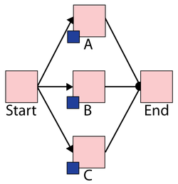
• The failure distributions of all three blocks follow a Weibull distribution with Beta = 1.5 and Eta = 1,000 hours.
• The repair distributions of the three blocks follow a Weibull distribution with Beta = 1.5 and Eta = 100 hours.
• After repair, the blocks are "as good as new."

There are three maintenance groups, 2_A, 2_B and 2_C, set as follows:

• Block A belongs to maintenance group 2_A.
  • It has a state change trigger.
    • The initial state is ON and the state upon repair is "Default OFF unless SCT overridden."
    • If any item from maintenance group 2_C goes down, then activate this block.

• Block B belongs to maintenance group 2_B.
  • It has a state change trigger.
    • The initial state is OFF and the state upon repair is "Default OFF unless SCT overridden."
    • If any item from maintenance group 2_A goes down, then activate this block.

• Block C belongs to maintenance group 2_C.
  • It has a state change trigger.
    • The initial state is OFF and the state upon repair is "Default OFF unless SCT overridden."
    • If any item from maintenance group 2_B goes down, then activate this block.

• All blocks A, B and C are as good as new after repair.

System Events

The system event log for a single run through the simulation algorithm is shown in the Block Up/Down plot below, and is as follows:

1. At 73 hours, Block A fails and activates Block B.
2. At 183 hours, Block B fails and activates Block C.
3. At 215 hours, Block B is done with repair. At this time, Block C is operating, so according to the settings, Block B is standby.
4. At 238 hours, Block A is done with repair. At this time, Block C is operating. Thus Block A is standby.
5. At 349 hours, Block C fails and activates Block A.
6. At 396 hours, Block A fails and activates Block B.
7. At 398 hours, Block C is done with repair. At this time, Block B is operating. Thus Block C is standby.
8. At 432 hours, Block A is done with repair. At this time, Block B is operating. Thus Block A is standby.
9. At 506 hours, Block B fails and activates Block C.
10. At 515 hours, Block B is done with repair and stays standby because Block C is operating.
11. At 536 hours, Block C fails and activates Block A.
12. At 560 hours, Block A fails and activates Block B.
13. At 575 hours, Block B fails and makes a request to activate Block C. However, Block C is under repair at the time. Thus when Block C is done with repair at 606 hours, the OFF setting is overridden and it is operating immediately.
14. At 661 hours, Block C fails and makes a request to activate Block A. However, Block A is under repair at the time. Thus when Block A is done with repair at 699 hours, the OFF setting is overridden and it is operating immediately.
15. Block B and Block C are done with repair at 682 hours and at 746 hours respectively. However, at these two time points, Block A is operating. Thus they are both standby upon repair according to the settings.

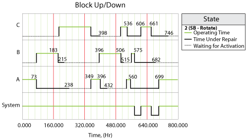
Consider a car with four regular tires (RF, LF, RR, LR) and a spare tire (SP). Assume that each tire can fail based on two failure modes, wear and puncture, and:

• The wear failure mode follows a Weibull distribution with Beta = 1.5, Eta = 600 hours.
• The puncture failure mode follows an exponential distribution with a mean of 2 months.
• Regardless of the failure mode, the repair duration (of both wear and puncture) follows a Weibull distribution with Beta = 1.5,Eta = 100 hours.
• If the tire fails due to wear, the tire is replaced with a new one (wear is repaired as-good-as-new).
• If the tire fails due to a puncture, it is patched up and placed back into service (repaired as-bad-as-old).
• When a primary tire (RF, LF, RR or LR) fails, it is replaced with the spare (SP) until that tire is restored. Once restored, the tire is put back in its original position and the spare is removed and put back for later use.

The purpose of this example is to illustrate the following options in State Change Triggers (SCT):

1. State Upon Repair: Always ON, Always OFF
2. Activate a block if any item from these associated maintenance group(s) goes down
3. Deactivate a block if any item from these associated maintenance group(s) is restored
4. Deactivate a block if any item from these associated maintenance group(s) goes down
5. Activate a block if any item from these associated maintenance group(s) is restored

BlockSim Solution

• To model this system, six diagrams are created: Car, Tire_LF, Tire_LR, Tire_RF, Tire_RR and Tire_SP with Car being the main diagram. Create the diagrams as follows:

1. First create diagram Tire_LF with two blocks in series. Block Wear_LF represents the Wear failure mode and Puncture_LF represents the Puncture failure mode for Tire_LF respectively.
   1. Block Wear_LF belongs to maintenance group "Wear_LF" and Block Puncture_LF belongs to maintenance group "Puncture_LF."
   2. Block Wear_LF has state change triggers; its initial state is ON, and the state upon repair is "Always ON." If any item from maintenance group "Puncture_LF" goes down, deactivate this block and if any item from maintenance group "Puncture_LF" is restored, activate this block.
   3. Block Puncture_LF has state change triggers; its initial state is ON, and the state upon repair is "Always ON." If any item from maintenance group "Wear_LF" goes down, deactivate this block and if any item from maintenance group "Wear_LF" is restored, activate this block.
      
2. Create the other three diagrams (Tire_LR, Tire_RF and Tire_RR) following the same logic.
3. In diagram Tire_SP, there are two blocks in series. Block Wear_SP represents the Wear failure mode and Puncture_SP represents the Puncture failure mode for the spare tire. Block Wear_SP belongs to maintenance group "Wear_SP" and Block Puncture_SP belongs to maintenance group "Puncture_SP."
   1. Block Wear_SP has state change triggers; its initial state is OFF, and the state upon repair is "Always OFF." If any item from maintenance group "Puncture_SP" goes down, deactivate this block and if any item from maintenance group "Puncture_SP" is restored, activate this block. If any item from maintenance group "Main Tires" goes down, activate this block and if any item from the maintenance group "Main Tires" is restored, deactivate this block. 
   2. Block Puncture_SP has state change triggers; its initial state is OFF, and the state upon repair is "Always OFF." If any item from maintenance group "Wear_SP" goes down, deactivate this block and if any item from maintenance group "Wear_SP" is restored, activate this block. If any item from maintenance group "Main Tires" goes down, activate this block and if any item from the maintenance group "Main Tires" is restored, deactivate this block.
      
4. In the diagram Car, there are five subdiagram blocks Tire_LF, Tire_LR, Tire_RF, Tire_RR and Tire_SP (each referencing/pointing to the diagram with the same names).
   1. In diagram Car, subdiagram blocks Tire_LF, Tire_LR, Tire_RF and Tire_RR belong to maintenance group "Main Tires."

Blocks Up/Down Plot

The system event log is shown in the figure below and is as follows (only blocks with failures are plotted):

1. At 46 hours, Block Wear_LR fails and brings down subdiagram Tire_LR. At the same time, it turns Block Puncture_LR OFF. Subdiagram Tire_LR goes down and activates Block Wear_SP and Puncture_SP, and subdiagram Spare is turned ON, too.
   
2. At 184 hours, Block Wear_LR is done with repair. According to the settings, it is always ON upon repair (is restored). The restoration of Block Wear_LR activates Block Puncture_LR and thus subdiagram Tire_LR is ON. The restoration of subdiagram Tire_LR deactivates Block Wear_SP and Puncture_SP, and subdiagram Tire_SP is turned OFF, too.
   
3. At 375 hours, Block Wear_RF fails and brings down subdiagram Tire_RF. At the same time, it turns Block Puncture_RF OFF. Subdiagram Tire_RF goes down and activates Block Wear_SP and Puncture_SP, and subdiagram Tire_SP is turned ON, too.
   
4. At 445 hours, Block Wear_RF is done with repair. According to the settings, it is always ON upon repair. The restoration of Block Wear_RF activates Block Puncture_RF and thus subdiagram Tire_RF is ON. The restoration of subdiagram Tire_RF deactivates Block Wear_SP and Puncture_SP, and subdiagram Tire_SP is turned OFF, too.
   
5. At 536 hours, Block Wear_LR fails again and brings down subdiagram Tire_LR. At the same time, it turns Block Puncture_LR OFF. Subdiagram Tire_LR goes down and activates Block Wear_SP and Puncture_SP, and the subdiagram Tire_SP is turned ON, too.
6. At 572 hours, Block Puncture_SP fails and brings down subdiagram Tire_SP. At the same time, it turns Block Wear_SP OFF. Subdiagram Tire_LR is already down at this time. Thus the system is down.
7. At 602 hours, Block Wear_LR is done with repair. According to the settings, it is always ON upon repair. The restoration of Block Wear_LR activates Block Puncture_LR and thus subdiagram Tire_LR is ON. The restoration of subdiagram Tire_LR should deactivate Block Wear_SP and Puncture_SP. However, Wear_SP is already OFF and Puncture_SP is already down at this time, thus nothing happens. The system is ON at this time due to the restoration of subdiagram Tire_LR.
8. At 617 hours, Block Puncture_SP is done with repair. According to the settings, it is always OFF upon repair.
9. At 686 hours, Block Puncture_LR fails and brings down subdiagram Tire_LR. At the same time, it turns Block Wear_LR OFF. Subdiagram Tire_LR goes down and activates Block Wear_SP and Puncture_SP, and the subdiagram Tire_SP is turned ON, too.
10. At 718 hours, Block Puncture_LR is done with repair. According to the settings, it is always ON upon repair. The restoration of Block Puncture_LR actives Block Wear_LR and thus subdiagram Tire_LR is ON. The restoration of subdiagram Tire_LR deactivates Block Wear_SP and Puncture_SP, and the subdiagram Tire_SP is turned OFF, too.

The purpose of this example is to illustrate how to model standby with delay using State Change Triggers (SCT).

Problem Statement

Three devices A, B and C are in parallel. 2 out of 3 are required to perform the task. Initially A and B are working and C is in standby status. If A or B fails, C will replace the failed one with some delay. After the failed device is restored, it will become a standby device. For example, if A fails, with 10 hours delay C will become active and replace A. After A is restored, it will become a standby device for B and C.

BlockSim Solution

The BlockSim modeling of this system is shown in the figure below.

In order to model the delay, three extra blocks AA, BB and CC are added to the diagram. Each of them fails every 10 hours (normal distribution with mean 10 hours and standard deviation 0.0000001 hours). They operate even if the system is down and repair durations for them are 0 (immediate repair). Block AA(BB/CC) belongs to maintenance group AA(BB/CC). They all have state change triggers. The initial state for each is OFF and the state upon repair is "Always OFF." If Block A (B/C) goes down, then activate Block AA (BB/CC).

Block A fails every 100 hours. It belongs to maintenance group A. It has state change triggers. The initial state is ON; the state upon repair is "Default OFF unless SCT overridden." If Block BB or Block CC goes down, Block A is activated.

Block B fails every 200 hours. It belongs to maintenance group B. It has state change triggers. The initial state is ON; the state upon repair is "Default OFF unless SCT overridden." If Block AA or Block CC goes down, Block B is activated.

Block C fails every 300 hours. It belongs to maintenance group C. It has state change triggers. The initial state is OFF; the state upon repair is "Default OFF unless SCT overridden." If Block BB or Block AA goes down, Block C is activated.

The repair duration for Blocks A, B and C is 30 hours.

Block Up/Down Plot

The system event log is shown in the figure below and is as follows:

1. At 100 hours, Block A fails and activates Block AA.
2. At 110 hours, Block AA fails and activates Block C.
3. At 230 hours, Block B fails and activates Block BB.
4. At 240 hours, Block BB fails and activates Block A.
5. At 340 hours, Block A fails and activates Block AA.
6. At 350 hours, Block AA fails and activates Block B.
7. ...

The purpose of this example is to illustrate how to use state change triggers (SCT) to model a system with two standby devices.

Problem Statement

Assume that there are four devices A, B, C and D in the system. The system begins with A and B as active devices and C and D as standby devices. At least 2 out of the 4 devices have to be in active status to assure that the system is working. If one of the active device fails, one of standby devices will be activated. After the active device is restored, it will become a standby device. For example, when A fails, C or D will be activated. After A finishes repair, it will become a standby device.

BlockSim Solution

It is easy to model this system with standby containers. However, standby containers have some limitations in other applications. Here we want to model this system with SCT. It is not possible to model this system directly with SCT, so we present an alternative solution which can approximate this system.

The logic is as follows: We will activate all standby devices whenever an active device fails. After activating all standby devices, we will check how many devices are in active status. If there are more than 2 devices in active status, we will deactivate some of them to assure that there are exactly two devices in active status at every moment. The drawback of this solution is that it will activate and deactivate the devices more times than we expected. For example, if A and B are active, then when A fails, it will activate C and D. After activating C and D it will detect that there are three devices in active status, so it will deactivate one of the three active devices: B, C or D. As we can see, it has the chance to deactivate B instead of C, which is not what we expected. If there is extra cost related to activation, this solution is not a good option.

In order to detect that there are more than two devices in active status, we have four subdiagram blocks: ABC, ABD, ACD and BCD. ABC contains mirror blocks A, B and C in series. The RBDs for the main diagram and subdiagram are as shown in the figures below.

Mirror group A includes Block A in the main diagram, Block A in subdiagram ABC, Block A in subdiagram ABD and Block A in subdiagram ACD.

Mirror group B includes Block B in the main diagram, Block B in subdiagram ABC, Block B in subdiagram ABD and Block B in subdiagram BCD.

Mirror group C includes Block C in the main diagram, Block C in subdiagram ABC, Block C in subdiagram BCD and Block C in subdiagram ACD.

Mirror group A includes Block D in the main diagram, Block D in subdiagram ABD, Block D in subdiagram ACD and Block D in subdiagram BCD.

All four blocks (A, B, C and D) follow a Weibull distribution with Beta = 1.5 and Eta = 100 hours for reliability and have CM with duration = 100 hours.

Block A belongs to maintenance group A. It has SCT with initial state ON and state upon repair "Default OFF unless SCT overridden." If any item from maintenance group B, C and D goes down, Block A is activated. If any item from maintenance group ABC is restored, we will deactivate Block A.

Block B belongs to maintenance group B. It has SCT with initial state ON and state upon repair "Default OFF unless SCT overridden." If any item from maintenance group A, C and D goes down, Block B is activated. If any item from maintenance group ABD is restored, we will deactivate Block B.

Block C belongs to maintenance group C. It has SCT with initial state OFF and state upon repair "Default OFF unless SCT overridden." If any item from maintenance group A, B and D goes down, Block C is activated. If any item from maintenance group ACD is restored, we will deactivate Block C.

Block D belongs to maintenance group D. It has SCT with initial state OFF and state upon repair "Default OFF unless SCT overridden." If any item from maintenance group A, B and C goes down, Block D is activated. If any item from maintenance group BCD is restored, we will deactivate Block D.

Subdiagram block ABC belongs to maintenance group ABC. The other three subdiagram blocks each belong to the maintenance group with the corresponding name.

System Events

The system event log for a single run through the simulation algorithm (simulation seed: 9)is shown in the Block Up/Down plot below, and is as follows:

1. At 26 hours, Block A fails. Block C and D are activated. However, there are three blocks in active status, thus Block D is deactivated immediately. 
2. At 126 hours, Block A finishes its repair. According to the settings, Block A is OFF as a standby device.
3. At 224 hours, Block C fails. Blocks A and D are activated. However, there are three blocks (A, B, and D) in active status, thus Block B is deactivated immediately. NOTICE: B should not be deactivated here, however we cannot control this. This is the drawback of this solution. If there is extra cost related to activation and deactivation, we are wasting resources by deactivating Block B. 
4. At 243 hours, Block A fails and activates Block B. 
5. At 248 hours, Block B fails and this failure tries to activate Blocks A and C. However, Blocks A and C are down at this time. This trigger event is on hold for Blocks A and C. After Block A and C finish their repair at 324 hours and 343 hours respectively, they are ON immediately.
6. At 343 hours, Block A finishes its repair. There is a trigger event on hold due to the failure of Block B at 248 hours. Block A is ON upon repair. At this time, there are three blocks in active status (Blocks A, C and D), thus Block C is deactivated immediately. This is another instance of wasting resources. The ideal case would be for Block A to be deactivated at this time.
7. At 408 hours, Block A fails and activates Blocks B and C. Since there are three blocks in active status, Block D is deactivated immediately to assure that only two blocks are in active status. 

Discussion

Even though the examples and explanations presented here are deterministic, the sequence of events and logic used to view the system is the same as the one that would be used during simulation. The difference is that the process would be repeated multiple times during simulation and the results presented would be the average results over the multiple runs.

Additionally, multiple metrics and results are presented and defined in this chapter. Many of these results can also be used to obtain additional metrics not explicitly given in BlockSim's Simulation Results Explorer. As an example, to compute mean availability with inspections but without PMs, the explicit downtimes given for each event could be used. Furthermore, all of the results given are for operating times starting at zero to a specified end time (although the components themselves could have been defined with a non-zero starting age). Results for a starting time other than zero could be obtained by running two simulations and looking at the difference in the detailed results where applicable. As an example, the difference in uptimes and downtimes can be used to determine availabilities for a specific time window.