Stress-Strength Analysis: Difference between revisions
Lisa Hacker (talk | contribs) No edit summary |
Kate Racaza (talk | contribs) No edit summary |
||
| Line 1: | Line 1: | ||
{{stress-strength analysis}} | ==Stress-Strength Analysis== | ||
===The Expected Probability=== | |||
Stress-strength analysis has been used in mechanical component design. The probability of failure is based on the probability of stress exceeding strength. The following equation is used to calculate the expected probability of failure, ''F'': | |||
<center><math>F=P[Stress\ge Strength]=\int_{0}^{\infty }{{{f}_{Strength}}(x)\cdot {{R}_{Stress}}(x)}dx</math></center> | |||
The expected probability of success or the expected reliability, ''R'' , is calculated as: | |||
<center><math>R=P[Stress\le Strength]=\int_{0}^{\infty }{{{f}_{Stress}}(x)\cdot {{R}_{Strength}}(x)}dx</math></center> | |||
The above calculation assumes both stress and strength are in the positive domain. For general cases, the expected reliability can be calculated using the following equation: | |||
<center><math>R=P[{{X}_{1}}\le {{X}_{2}}]=\frac{1}{{{F}_{1}}(U)-{{F}_{1}}(L)}\int_{L}^{U}{{{f}_{1}}(x)\cdot {{R}_{2}}(x)}dx</math></center> | |||
where: | |||
:: <math>L\le {{X}_{1}}\le U</math> | |||
::<math>\begin{align} | |||
& {{X}_{1}}:\text{ Stress } \\ | |||
& {{X}_{2}}:\text{ Strength } \\ | |||
\end{align}</math> | |||
<br> | |||
When U = infinite and L = 0, the above two equations are the same. | |||
===Confidence Intervals on the Probability=== | |||
Both the stress and strength distributions can be estimated from actual data or specified by engineers based on engineering knowledge or existing references. Based on the source of the distribution, there are two types of variation associated with the calculated probability: variation in the model parameters and variation in the probability values. Both are described next. | |||
'''Variation in Model Parameters''' | |||
If both the stress and strength distributions are estimated from data sets, then there are uncertainties associated with the estimated distribution parameters. These uncertainties will cause some degree of variation of the probability calculated from the stress-strength analysis. Therefore, we can use these uncertainties to estimate the confidence intervals on the calculated probability. To get the confidence intervals, we first calculate the variance of the reliability, <math>R</math>, using: | |||
<center> | |||
<math>Var\left[ R \right]=\int_{0}^{\infty }{Var\left[ {{f}_{1}}(x) \right]}{{\left[ {{R}_{2}}(x) \right]}^{2}}dx+{{\int_{0}^{\infty }{\left[ {{f}_{1}}(x) \right]}}^{2}}Var\left[ {{R}_{2}}(x) \right]dx</math> </center> | |||
Variance of <math>{{f}_{1}}(x)</math> and <math>{{R}_{2}}(x)</math> can be estimated from the Fisher Information Matrix. For details, please see [[Confidence Bounds]]. | |||
Once the variance of the expected reliability is obtained, the two-sided confidence intervals can be calculated using: | |||
<center><math>[\frac{R}{R+(1-R)w},\frac{R}{R+(1-R)/w}]</math></center> | |||
where: | |||
:: CL is the confidence level | |||
:: <math>\alpha</math> is 1-CL | |||
:: <math>w=\exp \{{{z}_{1-\alpha /2}}\sqrt{Var(R)}/[R(1-R)]\}</math> | |||
:: <math>{{Z}_{1-\alpha /2}}</math> is the <math>1-\alpha/2</math> percentile of a standard normal distribution. | |||
If the upper bound (U) and lower bound (L) are not infinite and 0, respectively, then the calculated variance of <math> R </math> is adjusted by <math>{{\left[ {1}/{\left( {{F}_{1}}(U)-{{F}_{1}}(L) \right)}\; \right]}^{2}}</math>. | |||
'''Variation in Probability Values''' | |||
Assume the distributions for stress and strength are known. From the stress-strength equation | |||
<center><math>R=P[Stress\le Strength]=\int_{0}^{\infty }{{{f}_{Stress}}(x)\cdot {{R}_{Strength}}(x)}dx</math></center> | |||
we know that the calculated reliability is the '''expected''' value of the probability that a strength value is larger than a stress value. Since both strength and stress are random variables from their distributions, the '''reliability''' is also a random variable. This can be explained using the following example. Let's first assume that stress is a fixed value of 567. The reliability then is: | |||
<center> | |||
<math>R(567)=\Pr (Strength>567)={{R}_{2}}(567)</math> | |||
</center> | |||
This is the reliability when the stress value is 567 and when the strength distribution is given. If stress is not a fixed value (i.e., it follows a distribution instead), then it can take values other than 567. For instance, if stress takes a value of 700, then we get another reliability value of <math>{R}(700)</math>. Since stress is a random variable, for any stress value <math>{x}_{i}</math>, there is a reliability value of | |||
<math>R({{x}_{i}})</math> calculated from the strength distribution. We will end up with many <math>R({{x}_{i}})</math>s or <math>R_{2}({{x}_{i}})</math>s. From these <math>R({{x}_{i}})</math>s, we can get the mean and variance of the reliability. In fact, its mean is the result from: | |||
<center><math>R=P[Stress\le Strength]=\int_{0}^{\infty }{{{f}_{Stress}}(x)\cdot {{R}_{Strength}}(x)}dx</math></center> | |||
and its variance is: | |||
<center> | |||
<math>\begin{align} | |||
& Var\left[ R \right]=Var\left[ {{R}_{2}}({{X}_{1}}) \right]=E\left[ {{R}_{2}}{{\left( {{X}_{1}} \right)}^{2}} \right]-{{\left( E\left[ {{R}_{2}}\left( {{X}_{1}} \right) \right] \right)}^{2}} \\ | |||
& =\int_{0}^{\infty }{{{f}_{1}}(x){{\left[ {{R}_{2}}(x) \right]}^{2}}dx}-{{\left( E\left[ {{R}_{2}}\left( {{X}_{1}} \right) \right] \right)}^{2}} \\ | |||
& =\int_{0}^{\infty }{{{f}_{1}}(x){{\left[ {{R}_{2}}(x) \right]}^{2}}dx}-{{\left( R \right)}^{2}} \\ | |||
\end{align}</math></center> | |||
where ''R'' is the expected value of the reliability. | |||
Once the variance of the expected reliability is obtained, the two-sided confidence intervals can be calculated using: | |||
<center><math>[\frac{R}{R+(1-R)w},\frac{R}{R+(1-R)/w}]</math></center> | |||
where: | |||
:: CL is the confidence level | |||
:: <math>\alpha</math> is 1-CL | |||
:: <math>w=\exp \{{{z}_{1-\alpha /2}}\sqrt{Var(R)}/[R(1-R)]\}</math> | |||
:: <math>{{Z}_{1-\alpha /2}}</math> is the <math>1-\alpha/2</math> percentile of a standard normal distribution | |||
If the upper bound (U) and lower bound (L) are not infinite and 0, the above calculated variance of ''R'' is adjusted by <math>{{\left[ {1}/{\left( {{F}_{1}}(U)-{{F}_{1}}(L) \right)}\; \right]}^{2}}</math>. | |||
'''Example 1:''' | |||
{{Example: Stress-Strength Analysis with Parameter Uncertainty}} | |||
===Stress-Strength Analysis in Design for Reliability=== | |||
As we know, the expected reliability is called from the following stress-strength calculation: | |||
<center><math>R=P[Stress\le Strength]=\int_{0}^{\infty }{{{f}_{Stress}}(x)\cdot {{R}_{Strength}}(x)}dx</math></center> | |||
The stress distribution is usually estimated from customer usage data, such as the mileage per year of a passenger car or the load distribution for a beam. The strength distribution, on the other hand, is affected by the material used in the component, the geometric dimensions and the manufacturing process. | |||
Because the stress distribution can be estimated from customer usage data, we can assume that <math>{f}_{Stress} </math> is known. Therefore, for a given reliability goal, the strength distribution <math> {R}_{Strength}</math> is the only unknown in the given equation. The factors that affect the strength distribution can be adjusted to obtain a strength distribution that meets the reliability goal. The following example shows how to use the Target Reliability Parameter Estimator tool in the stress-strength folio to obtain the parameters for a strength distribution that will meet a specified reliability goal. | |||
'''Example 2:''' | |||
{{Example: Stress-Strength Analysis for Determing Strength Distribution}} | |||
Revision as of 09:44, 29 June 2012
Stress-Strength Analysis
The Expected Probability
Stress-strength analysis has been used in mechanical component design. The probability of failure is based on the probability of stress exceeding strength. The following equation is used to calculate the expected probability of failure, F:
The expected probability of success or the expected reliability, R , is calculated as:
The above calculation assumes both stress and strength are in the positive domain. For general cases, the expected reliability can be calculated using the following equation:
where:
- [math]\displaystyle{ L\le {{X}_{1}}\le U }[/math]
- [math]\displaystyle{ \begin{align} & {{X}_{1}}:\text{ Stress } \\ & {{X}_{2}}:\text{ Strength } \\ \end{align} }[/math]
When U = infinite and L = 0, the above two equations are the same.
Confidence Intervals on the Probability
Both the stress and strength distributions can be estimated from actual data or specified by engineers based on engineering knowledge or existing references. Based on the source of the distribution, there are two types of variation associated with the calculated probability: variation in the model parameters and variation in the probability values. Both are described next.
Variation in Model Parameters
If both the stress and strength distributions are estimated from data sets, then there are uncertainties associated with the estimated distribution parameters. These uncertainties will cause some degree of variation of the probability calculated from the stress-strength analysis. Therefore, we can use these uncertainties to estimate the confidence intervals on the calculated probability. To get the confidence intervals, we first calculate the variance of the reliability, [math]\displaystyle{ R }[/math], using:
Variance of [math]\displaystyle{ {{f}_{1}}(x) }[/math] and [math]\displaystyle{ {{R}_{2}}(x) }[/math] can be estimated from the Fisher Information Matrix. For details, please see Confidence Bounds.
Once the variance of the expected reliability is obtained, the two-sided confidence intervals can be calculated using:
where:
- CL is the confidence level
- [math]\displaystyle{ \alpha }[/math] is 1-CL
- [math]\displaystyle{ w=\exp \{{{z}_{1-\alpha /2}}\sqrt{Var(R)}/[R(1-R)]\} }[/math]
- [math]\displaystyle{ {{Z}_{1-\alpha /2}} }[/math] is the [math]\displaystyle{ 1-\alpha/2 }[/math] percentile of a standard normal distribution.
If the upper bound (U) and lower bound (L) are not infinite and 0, respectively, then the calculated variance of [math]\displaystyle{ R }[/math] is adjusted by [math]\displaystyle{ {{\left[ {1}/{\left( {{F}_{1}}(U)-{{F}_{1}}(L) \right)}\; \right]}^{2}} }[/math].
Variation in Probability Values
Assume the distributions for stress and strength are known. From the stress-strength equation
we know that the calculated reliability is the expected value of the probability that a strength value is larger than a stress value. Since both strength and stress are random variables from their distributions, the reliability is also a random variable. This can be explained using the following example. Let's first assume that stress is a fixed value of 567. The reliability then is:
[math]\displaystyle{ R(567)=\Pr (Strength\gt 567)={{R}_{2}}(567) }[/math]
This is the reliability when the stress value is 567 and when the strength distribution is given. If stress is not a fixed value (i.e., it follows a distribution instead), then it can take values other than 567. For instance, if stress takes a value of 700, then we get another reliability value of [math]\displaystyle{ {R}(700) }[/math]. Since stress is a random variable, for any stress value [math]\displaystyle{ {x}_{i} }[/math], there is a reliability value of
[math]\displaystyle{ R({{x}_{i}}) }[/math] calculated from the strength distribution. We will end up with many [math]\displaystyle{ R({{x}_{i}}) }[/math]s or [math]\displaystyle{ R_{2}({{x}_{i}}) }[/math]s. From these [math]\displaystyle{ R({{x}_{i}}) }[/math]s, we can get the mean and variance of the reliability. In fact, its mean is the result from:
and its variance is:
where R is the expected value of the reliability.
Once the variance of the expected reliability is obtained, the two-sided confidence intervals can be calculated using:
where:
- CL is the confidence level
- [math]\displaystyle{ \alpha }[/math] is 1-CL
- [math]\displaystyle{ w=\exp \{{{z}_{1-\alpha /2}}\sqrt{Var(R)}/[R(1-R)]\} }[/math]
- [math]\displaystyle{ {{Z}_{1-\alpha /2}} }[/math] is the [math]\displaystyle{ 1-\alpha/2 }[/math] percentile of a standard normal distribution
If the upper bound (U) and lower bound (L) are not infinite and 0, the above calculated variance of R is adjusted by [math]\displaystyle{ {{\left[ {1}/{\left( {{F}_{1}}(U)-{{F}_{1}}(L) \right)}\; \right]}^{2}} }[/math].
Example 1:
Assume that the stress distribution for a component is known to be a Weibull distribution with beta = 3 and eta = 2000. For the current design, the strength distribution is also a Weibull distribution with beta =1.5 and eta=4000. Evaluate the current reliability of the component. If the reliability does not meet the target reliability of 90%, determine what parameters would be required for the strength distribution in order to meet the specified target.
Solution
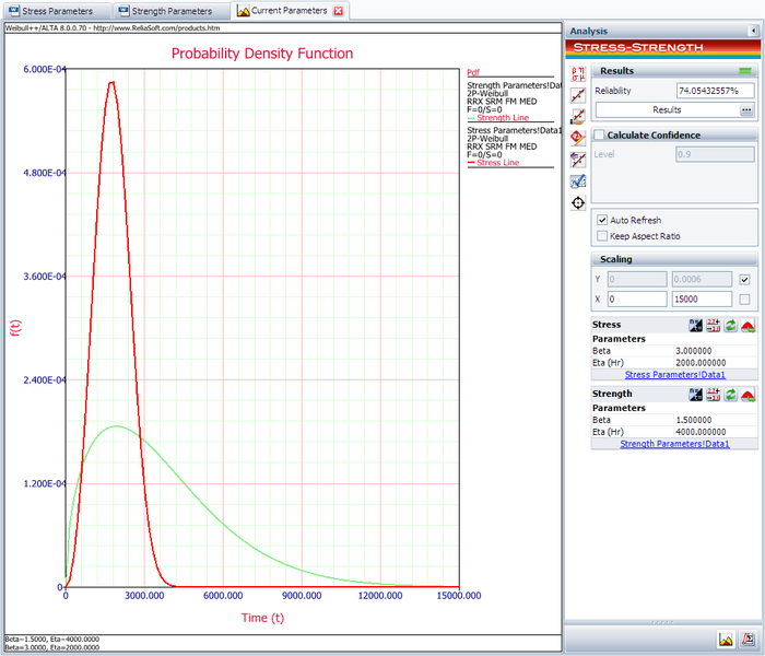
The following picture shows the stress-strength tool and the calculated reliability of the current design.
The result shows that the current reliability is about 74.0543%, which is below the target value of 90%. We need to use the Target Reliability Parameter Estimator to determine the parameters for the strength distribution that, when compared against the stress distribution, would result in the target reliability.
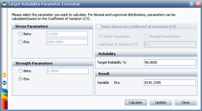
The following picture shows the Target Reliability Parameter Estimator window. In the Strength Parameters area, select eta. Set the Target Reliability to 90% and click Calculate. The calculated eta is 8192.2385 hours.
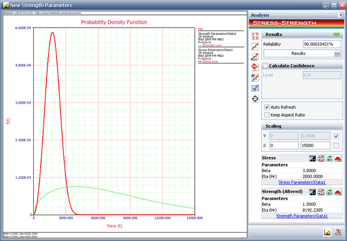
Click Update to perform the stress-strength analysis again using the altered parameters for the strength distribution. The following plot shows that the calculated reliability is 90%. Therefore, in order to meet the reliability requirement, the component must be redesigned such that the eta parameter of the strength distribution is at least 8192.2385 hours.
Stress-Strength Analysis in Design for Reliability
As we know, the expected reliability is called from the following stress-strength calculation:
The stress distribution is usually estimated from customer usage data, such as the mileage per year of a passenger car or the load distribution for a beam. The strength distribution, on the other hand, is affected by the material used in the component, the geometric dimensions and the manufacturing process.
Because the stress distribution can be estimated from customer usage data, we can assume that [math]\displaystyle{ {f}_{Stress} }[/math] is known. Therefore, for a given reliability goal, the strength distribution [math]\displaystyle{ {R}_{Strength} }[/math] is the only unknown in the given equation. The factors that affect the strength distribution can be adjusted to obtain a strength distribution that meets the reliability goal. The following example shows how to use the Target Reliability Parameter Estimator tool in the stress-strength folio to obtain the parameters for a strength distribution that will meet a specified reliability goal.
Example 2:
Assume that the stress distribution for a component is known to be a Weibull distribution with beta = 3 and eta = 2000. For the current design, the strength distribution is also a Weibull distribution with beta =1.5 and eta=4000. Evaluate the current reliability of the component. If the reliability does not meet the target reliability of 90%, determine what parameters would be required for the strength distribution in order to meet the specified target.
Solution
The following picture shows the stress-strength tool and the calculated reliability of the current design.
The result shows that the current reliability is about 74.0543%, which is below the target value of 90%. We need to use the Target Reliability Parameter Estimator to determine the parameters for the strength distribution that, when compared against the stress distribution, would result in the target reliability.
The following picture shows the Target Reliability Parameter Estimator window. In the Strength Parameters area, select eta. Set the Target Reliability to 90% and click Calculate. The calculated eta is 8192.2385 hours.
Click Update to perform the stress-strength analysis again using the altered parameters for the strength distribution. The following plot shows that the calculated reliability is 90%. Therefore, in order to meet the reliability requirement, the component must be redesigned such that the eta parameter of the strength distribution is at least 8192.2385 hours.


