Template:2 parameter exponential distribution RRY example: Difference between revisions
No edit summary |
No edit summary |
||
| Line 121: | Line 121: | ||
::<math>\hat{\lambda }=0.0271\text{ fr/hr },\hat{\gamma }=10.1348\text{ hr },\hat{\rho }=-0.9679</math> | ::<math>\hat{\lambda }=0.0271\text{ fr/hr },\hat{\gamma }=10.1348\text{ hr },\hat{\rho }=-0.9679</math> | ||
[[Image:Exponential Example 2 Data Folio.png|thumb|center| | [[Image:Exponential Example 2 Data Folio.png|thumb|center|550px|]] | ||
Please note that the user must deselect the '''Reset if | Please note that the user must deselect the '''Reset if location parameter > T1 on Exponential''' option on the Calculations page of the Application Setup window. | ||
The probability plot can be obtained simply by clicking the '''Plot''' icon. | The probability plot can be obtained simply by clicking the '''Plot''' icon. | ||
[[Image:Exponential Example 2 Plot.png|thumb|center| | [[Image:Exponential Example 2 Plot.png|thumb|center|550px|]] | ||
Revision as of 02:38, 6 August 2012
2 Parameter Exponential Distribution RRY
2 Paramter Exponential Distribution RRY
Fourteen units were being reliability tested and the following life test data were obtained:
| Table - Life Test Data | |
| Data point index | Time-to-failure |
|---|---|
| 1 | 5 |
| 2 | 10 |
| 3 | 15 |
| 4 | 20 |
| 5 | 25 |
| 6 | 30 |
| 7 | 35 |
| 8 | 40 |
| 9 | 50 |
| 10 | 60 |
| 11 | 70 |
| 12 | 80 |
| 13 | 90 |
| 14 | 100 |
Assuming that the data follow a two-parameter exponential distribution, estimate the parameters and determine the correlation coefficient, [math]\displaystyle{ \rho }[/math], using rank regression on Y.
Solution
Construct the following table, as shown next.
The median rank values ( [math]\displaystyle{ F({{t}_{i}}) }[/math] ) can be found in rank tables or they can be estimated using the Quick Statistical Reference in Weibull++.
Given the values in the table above, calculate [math]\displaystyle{ \hat{a} }[/math] and [math]\displaystyle{ \hat{b} }[/math]:
- [math]\displaystyle{ \begin{align} \hat{b}= & \frac{\underset{i=1}{\overset{14}{\mathop{\sum }}}\,{{t}_{i}}{{y}_{i}}-(\underset{i=1}{\overset{14}{\mathop{\sum }}}\,{{t}_{i}})(\underset{i=1}{\overset{14}{\mathop{\sum }}}\,{{y}_{i}})/14}{\underset{i=1}{\overset{14}{\mathop{\sum }}}\,t_{i}^{2}-{{(\underset{i=1}{\overset{14}{\mathop{\sum }}}\,{{t}_{i}})}^{2}}/14} \\ \\ \hat{b}= & \frac{-927.4899-(630)(-13.2315)/14}{40,600-{{(630)}^{2}}/14} \end{align} }[/math]
or:
- [math]\displaystyle{ \hat{b}=-0.02711 }[/math]
and:
- [math]\displaystyle{ \hat{a}=\overline{y}-\hat{b}\overline{t}=\frac{\underset{i=1}{\overset{N}{\mathop{\sum }}}\,{{y}_{i}}}{N}-\hat{b}\frac{\underset{i=1}{\overset{N}{\mathop{\sum }}}\,{{t}_{i}}}{N} }[/math]
or:
- [math]\displaystyle{ \hat{a}=\frac{-13.2315}{14}-(-0.02711)\frac{630}{14}=0.2748 }[/math]
Therefore:
- [math]\displaystyle{ \hat{\lambda }=-\hat{b}=-(-0.02711)=0.02711\text{ failures/hour} }[/math]
and:
- [math]\displaystyle{ \hat{\gamma }=\frac{\hat{a}}{\hat{\lambda }}=\frac{0.2748}{0.02711} }[/math]
or:
- [math]\displaystyle{ \hat{\gamma }=10.1365\text{ hours} }[/math]
Then:
- [math]\displaystyle{ f(t)=(0.02711)\cdot {{e}^{-0.02711(T-10.136)}} }[/math]
The correlation coefficient can be estimated using equation for calculating the correlation coefficient:
- [math]\displaystyle{ \hat{\rho }=-0.9679 }[/math]
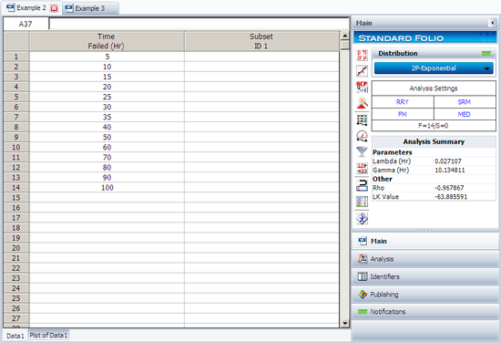
This example can be repeated using Weibull++, choosing two-parameter exponential and rank regression on Y (RRY), as shown in the figure on the following page.
The estimated parameters and the correlation coefficient using Weibull++ were found to be:
- [math]\displaystyle{ \hat{\lambda }=0.0271\text{ fr/hr },\hat{\gamma }=10.1348\text{ hr },\hat{\rho }=-0.9679 }[/math]
Please note that the user must deselect the Reset if location parameter > T1 on Exponential option on the Calculations page of the Application Setup window.
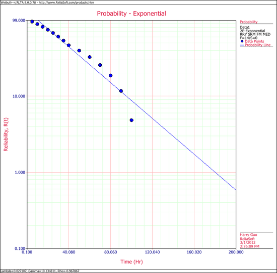
The probability plot can be obtained simply by clicking the Plot icon.

