Template:Automotive Step-Stress Example
Automotive Step-Stress Example
Consider a test in which multiple stresses were applied simultaneously to a particular automotive part in order to precipitate failures more quickly than they would occur under normal use conditions. The engineers responsible for the test were able to quantify the combination of applied stresses in terms of a "percentage stress" as compared to typical stress levels (or assumed field conditions). In this scenario, the typical stress (field or use stress) was defined as 100% and any combination of the test stresses was quantified as a percentage over the typical stress. For example, if the combination of stresses on test was determined to be two times higher than typical conditions, then the stress on test was said to be at 200%.
The test was set up and run as a step-stress test (i.e. the stresses were increased in a stepwise fashion) and the time on test was measured in hours. The step-stress profile used was as follows: until 200 hours, the equivalent applied stress was 125%; from 200 to 300 hrs, it was 175%; from 300 to 350 hrs, it was 200% and from 350 to 375 hrs, it was 250%. The test was terminated after 375 hours and any units that were still running after that point were right-censored (suspended).
Additionally, and based on prior analysis/knowledge, the engineers also stated that each hour on test under normal use conditions (i.e., at 100% stress measure) was equivalent to approximately 100 miles of normal driving. The test was conducted and the following times-to-failure and times-to-suspension under the stated step-stress profile were observed (note that + indicates a non-failed unit, i.e., suspension): 252, 280, 320, 328, 335, 354, 361, 362, 368, 375+, 375+, 375+.
After performing failure analysis on the failed parts, it was determined that the failure that occurred at 328 hrs was due to mechanisms other than the ones considered. That data point was therefore identified as a suspension in the currently analysis. The modified data set for this analysis was: 252, 280, 320, 328+, 335, 354, 361, 362, 368, 375+, 375+, 375+.
The test objective was to estimate the [math]\displaystyle{ B1 }[/math] life for the part (i.e. time at which reliability is equal to 99%) at the typical operating conditions (i.e., Stress=100%), in miles.
Solution
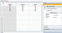
Utilizing ALTA, the analyst first created a Standard Folio for non-grouped time-to-failure and time-to-suspension data and added a Stress Profile under Tools in the Project Manager to define the stress profile, as shown next.
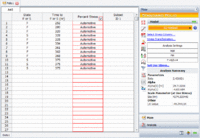
Once the profile was defined, the analyst entered the observed times, their state (i.e., failed F or non-failed S) and a reference to the profile used in the ALTA Standard Folio. The analyst selected the cumulative damage life-stress relationship (to use a time-varying stress) based on a power model (since the effect of the stress was deemed to be mechanical and more appropriately modeled by a power function). The Weibull distribution was selected as the underlying life distribution. Additionally, note that the use stress was set to 100 and all results were then extrapolated to the typical stress level. The Standard Folio and the selected model is shown next.
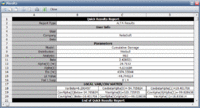
The estimated parameters are shown next.
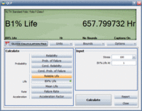
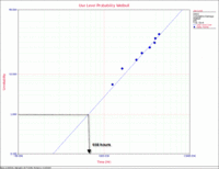
The last part remaining was to determine the [math]\displaystyle{ B1 }[/math] life at the part's use stress level. Using the QCP, the [math]\displaystyle{ B1 }[/math] life was found to be 658 hours, as shown next.
Based on the given multiplier, the [math]\displaystyle{ B1 }[/math] life in miles would then be 658 test-hr*100 (miles/test-hr)= 65,800 miles.
The [math]\displaystyle{ B1 }[/math] life can also be obtained from the use level probability plot, as shown next.
