Template:Aw characteristics: Difference between revisions
Chuck Smith (talk | contribs) |
Chuck Smith (talk | contribs) |
||
| Line 79: | Line 79: | ||
Eta (<span class="texhtml">η</span>) is called the scale parameter of the Weibull distribution. The parameter <span class="texhtml">η</span> has the same units as <span class="texhtml">''T''</span>, such as hours, miles, cycles, actuations, etc. | Eta (<span class="texhtml">η</span>) is called the scale parameter of the Weibull distribution. The parameter <span class="texhtml">η</span> has the same units as <span class="texhtml">''T''</span>, such as hours, miles, cycles, actuations, etc. | ||
<br> [[Image:ALTA4.7.png|center| | <br> [[Image:ALTA4.7.png|center|200px]] <br> | ||
:*A change in the scale parameter <span class="texhtml">η</span> has the same effect on the distribution as a change of the abscissa scale. | :*A change in the scale parameter <span class="texhtml">η</span> has the same effect on the distribution as a change of the abscissa scale. | ||
Revision as of 16:05, 26 April 2012
Characteristics
The characteristics of the 2-parameter Weibull distribution can be exemplified by examining the two parameters, beta, [math]\displaystyle{ \beta , }[/math] and eta, [math]\displaystyle{ \eta , }[/math] and the effect they have on the [math]\displaystyle{ pdf, }[/math] reliability and failure rate functions.
Looking at β
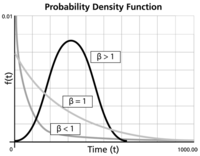
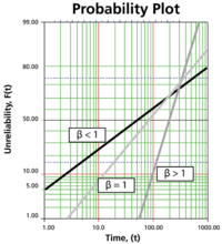
Beta (β) is called the shape parameter or slope of the Weibull distribution. Changing the value of β forces a change in the shape of the pdf as shown in the next figure. In addition, when the cdf is plotted on Weibull probability paper, a change in beta is a change in the slope of the distribution on Weibull probability paper.
Effects of β on the pdf
- For 0 < β < 1 , the failure rate decreases with time and:
- As [math]\displaystyle{ T\to 0, }[/math] [math]\displaystyle{ f(T)\to \infty }[/math].
- As [math]\displaystyle{ T\to \infty }[/math] , [math]\displaystyle{ f(T)\to 0 }[/math].
- f(T) decreases monotonically and is convex as T increases.
- The mode is non-existent.
- For β = 1, it becomes the exponential distribution, as a special case,
- or:
- [math]\displaystyle{ f(T)=\frac{1}{\eta }{{e}^{-\tfrac{T}{\eta }}};\text{ }\eta \gt 0,T\ge 0 }[/math]
- where [math]\displaystyle{ \tfrac{1}{\eta }=\lambda = }[/math] chance, useful life, or failure rate.
- For β > 1, f(T), the Weibull distribution assumes wear-out type shapes (i.e., the failure rate increases with time) and:
- f(T) = 0 at T = 0 .
- f(T) increases as [math]\displaystyle{ T\to \tilde{T} }[/math] (mode) and decreases thereafter.
- For β = 2 it becomes the Rayleigh distribution as a special case. For β < 2.6, the Weibull pdf is positively skewed (has a right tail). For 2.6 < β < 3.7, its coefficient of skewness approaches zero (no tail). Consequently, it may approximate the normal pdf, and for β > 3.7 it is negatively skewed (left tail).
- The parameter β is a pure number (i.e., it is dimensionless).
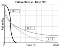
Effects of β on the Reliability Function and the cdf
- R(T) decreases sharply and monotonically for 0 < β < 1. It is convex and decreases less sharply for the same β.
- For β = 1 and the same η, R(T) decreases monotonically but less sharply than for 0 < β < 1, and it is convex.
- For β > 1, R(T) decreases as T increases but less sharply than before. As wear-out sets in, it decreases sharply and goes through an inflection point.
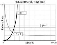
Effects of β on the Failure Rate Function
- The Weibull failure rate for 0 < β < 1 is unbounded at T = 0. The failure rate, λ(T), decreases thereafter monotonically and is convex, approaching the value of zero as [math]\displaystyle{ T\to \infty }[/math] or [math]\displaystyle{ \lambda (\infty )=0 }[/math]. This behavior makes it suitable for representing the failure rate of units exhibiting early-type failures, for which the failure rate decreases with age. When such behavior is encountered, one or more of the following conclusions can be drawn:
- Burn-in testing and/or environmental stress screening are not well implemented.
- There are problems in the production line.
- There is inadequate quality control.
- There are packaging and transit problems.
- For β = 1, λ(T) yields a constant value of [math]\displaystyle{ \tfrac{1}{\eta } }[/math] , or:
- [math]\displaystyle{ \lambda (T)=\lambda =\frac{1}{\eta } }[/math]
This makes it suitable for representing the failure rate of chance-type failures and the useful life period failure rate of units.
- For β > 1, λ(T) increases as T increases and becomes suitable for representing the failure rate of units exhibiting wear-out type failures. For 1 < β < 2, the λ(T) curve is concave. Consequently, the failure rate increases at a decreasing rate as T increases.
- For β = 2, or for the Rayleigh distribution case, the failure rate function is given by:
- [math]\displaystyle{ \lambda (T)=\frac{2}{\eta }\left( \frac{T}{\eta } \right) }[/math]
Hence there emerges a straight line relationship between λ(T) and T, starting at a value of λ(T) = 0 at T = 0 and increasing thereafter with a slope of [math]\displaystyle{ \tfrac{2}{{{\eta }^{2}}} }[/math] . Consequently, the failure rate increases at a constant rate as T increases. Furthermore, if η = 1 the slope becomes equal to 2, and λ(T) becomes a straight line which passes through the origin with a slope of 2.
- When β > 2 the λ(T) curve is convex, with its slope increasing as T increases. Consequently, the failure rate increases at an increasing rate as T increases, indicating wear-out life.
Looking at η
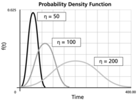
Eta (η) is called the scale parameter of the Weibull distribution. The parameter η has the same units as T, such as hours, miles, cycles, actuations, etc.
- A change in the scale parameter η has the same effect on the distribution as a change of the abscissa scale.
- If η is increased while β is kept the same, the distribution gets stretched out to the right and its height decreases, while maintaining its shape and location.
- If η is decreased while β is kept the same, the distribution gets pushed in toward the left (i.e. toward its beginning, or 0) and its height increases.
