Template:Aw probability plotting: Difference between revisions
| Line 33: | Line 33: | ||
\end{matrix}</math></center> | \end{matrix}</math></center> | ||
<br> | <br> | ||
:• On a Weibull probability paper, plot the times and their corresponding ranks. | :• On a Weibull probability paper, plot the times and their corresponding ranks. The next figure displays an example of a Weibull probability paper. | ||
<br> | <br> | ||
[[Image:ALTA4.8.gif|thumb|center|300px|Sample Weibull probability paper.]] | [[Image:ALTA4.8.gif|thumb|center|300px|Sample Weibull probability paper.]] | ||
<br> | <br> | ||
<br> | <br> | ||
:• Draw the best possible straight line through the plotted points | :• Draw the best possible straight line through the plotted points. | ||
:• Obtain the slope of this line by drawing a line, parallel to the one just obtained, through the slope indicator. This value is the estimate of the shape parameter <math>\widehat{\beta }</math> . In this case <math>\widehat{\beta }=1.4</math> . | :• Obtain the slope of this line by drawing a line, parallel to the one just obtained, through the slope indicator. This value is the estimate of the shape parameter <math>\widehat{\beta }</math> . In this case <math>\widehat{\beta }=1.4</math> . | ||
:• At the <math>Q(t)=63.2%</math> ordinate point, draw a straight horizontal line until this line intersects the fitted straight line. Draw a vertical line through this intersection until it crosses the abscissa. The value at the intersection of the abscissa is the estimate of <math>\widehat{\eta }</math> . For this case <math>\widehat{\eta }=76</math> hr. (This is always at 63.2% since <math>Q(T)=1-{{e}^{-{{(\tfrac{\eta }{\eta })}^{\beta }}}}=1-{{e}^{-1}}=0.632=63.2%).</math> | :• At the <math>Q(t)=63.2%</math> ordinate point, draw a straight horizontal line until this line intersects the fitted straight line. Draw a vertical line through this intersection until it crosses the abscissa. The value at the intersection of the abscissa is the estimate of <math>\widehat{\eta }</math> . For this case <math>\widehat{\eta }=76</math> hr. (This is always at 63.2% since <math>Q(T)=1-{{e}^{-{{(\tfrac{\eta }{\eta })}^{\beta }}}}=1-{{e}^{-1}}=0.632=63.2%).</math> | ||
| Line 44: | Line 44: | ||
[[Image:ALTA4.9.gif|thumb|center|300px|Probability plot for Example 3.]] | [[Image:ALTA4.9.gif|thumb|center|300px|Probability plot for Example 3.]] | ||
<br> | <br> | ||
Now any reliability value for any mission time <math>t</math> can be obtained. For example, the reliability for a mission of 15 hr, or any other time, can now be obtained either from the plot or analytically | Now any reliability value for any mission time <math>t</math> can be obtained. For example, the reliability for a mission of 15 hr, or any other time, can now be obtained either from the plot or analytically. | ||
To obtain the value from the plot, draw a vertical line from the abscissa, at <math>t=15</math> hr, to the fitted line. Draw a horizontal line from this intersection to the ordinate and read <math>Q(t)</math> , in this case <math>Q(t=15)=9.8%</math> . Thus, <math>R(t=15)=1-Q(t)=90.2%</math> . This can also be obtained analytically from the Weibull reliability function since both of the parameters are known. | To obtain the value from the plot, draw a vertical line from the abscissa, at <math>t=15</math> hr, to the fitted line. Draw a horizontal line from this intersection to the ordinate and read <math>Q(t)</math> , in this case <math>Q(t=15)=9.8%</math> . Thus, <math>R(t=15)=1-Q(t)=90.2%</math> . This can also be obtained analytically from the Weibull reliability function since both of the parameters are known. | ||
Revision as of 00:35, 7 February 2012
Probability Plotting
One method of calculating the parameters of the Weibull distribution is by using probability plotting. To better illustrate this procedure, consider the following example [18].
Example 3
Let's assume six identical units are being reliability tested at the same application and operation stress levels. All of these units fail during the test after operating the following times (in hours), [math]\displaystyle{ {{T}_{i}} }[/math] : 93, 34, 16, 120, 53 and 75.
The steps for determining the parameters of the Weibull [math]\displaystyle{ pdf }[/math] representing the data, using probability plotting, are as follows:
- • Rank the times-to-failure in ascending order as shown next.
- • Obtain their median rank plotting positions. The times-to-failure, with their corresponding median ranks, are shown next.
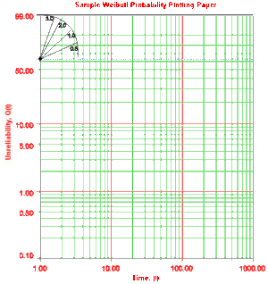
- • On a Weibull probability paper, plot the times and their corresponding ranks. The next figure displays an example of a Weibull probability paper.
- • Draw the best possible straight line through the plotted points.
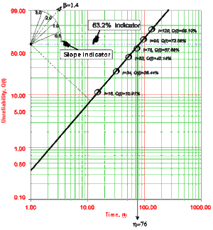
- • Obtain the slope of this line by drawing a line, parallel to the one just obtained, through the slope indicator. This value is the estimate of the shape parameter [math]\displaystyle{ \widehat{\beta } }[/math] . In this case [math]\displaystyle{ \widehat{\beta }=1.4 }[/math] .
- • At the [math]\displaystyle{ Q(t)=63.2% }[/math] ordinate point, draw a straight horizontal line until this line intersects the fitted straight line. Draw a vertical line through this intersection until it crosses the abscissa. The value at the intersection of the abscissa is the estimate of [math]\displaystyle{ \widehat{\eta } }[/math] . For this case [math]\displaystyle{ \widehat{\eta }=76 }[/math] hr. (This is always at 63.2% since [math]\displaystyle{ Q(T)=1-{{e}^{-{{(\tfrac{\eta }{\eta })}^{\beta }}}}=1-{{e}^{-1}}=0.632=63.2%). }[/math]
Now any reliability value for any mission time [math]\displaystyle{ t }[/math] can be obtained. For example, the reliability for a mission of 15 hr, or any other time, can now be obtained either from the plot or analytically.
To obtain the value from the plot, draw a vertical line from the abscissa, at [math]\displaystyle{ t=15 }[/math] hr, to the fitted line. Draw a horizontal line from this intersection to the ordinate and read [math]\displaystyle{ Q(t) }[/math] , in this case [math]\displaystyle{ Q(t=15)=9.8% }[/math] . Thus, [math]\displaystyle{ R(t=15)=1-Q(t)=90.2% }[/math] . This can also be obtained analytically from the Weibull reliability function since both of the parameters are known.
- [math]\displaystyle{ R(t=15)={{e}^{-{{\left( \tfrac{15}{\eta } \right)}^{\beta }}}}={{e}^{-{{\left( \tfrac{15}{76} \right)}^{1.4}}}}=90.2%. }[/math]

