Template:Characteristics of the gumbel distribution: Difference between revisions
Jump to navigation
Jump to search
| Line 7: | Line 7: | ||
:* As <math>\mu </math> increases, the <math>pdf</math> is shifted to the right. | :* As <math>\mu </math> increases, the <math>pdf</math> is shifted to the right. | ||
[[Image: | [[Image:WB.16 gumbel pdf.png|center|400px| ]] | ||
:* As <math>\sigma </math> increases, the <math>pdf</math> spreads out and becomes shallower. | :* As <math>\sigma </math> increases, the <math>pdf</math> spreads out and becomes shallower. | ||
| Line 13: | Line 13: | ||
:* For <math>T=\pm \infty ,</math> <math>pdf=0.</math> For <math>T=\mu </math> , the <math>pdf</math> reaches its maximum point <math>\frac{1}{\sigma e}</math> | :* For <math>T=\pm \infty ,</math> <math>pdf=0.</math> For <math>T=\mu </math> , the <math>pdf</math> reaches its maximum point <math>\frac{1}{\sigma e}</math> | ||
[[Image: | [[Image:WB.16 effect of sigma.png|center|400px| ]] | ||
:* The points of inflection of the <math>pdf</math> graph are <math>T=\mu \pm \sigma \ln (\tfrac{3\pm \sqrt{5}}{2})</math> or <math>T\approx \mu \pm \sigma 0.96242</math> . | :* The points of inflection of the <math>pdf</math> graph are <math>T=\mu \pm \sigma \ln (\tfrac{3\pm \sqrt{5}}{2})</math> or <math>T\approx \mu \pm \sigma 0.96242</math> . | ||
:* If times follow the Weibull distribution, then the logarithm of times follow a Gumbel distribution. If <math>{{t}_{i}}</math> follows a Weibull distribution with <math>\beta </math> and <math>\eta </math> , then the <math>Ln({{t}_{i}})</math> follows a Gumbel distribution with <math>\mu =\ln (\eta )</math> and <math>\sigma =\tfrac{1}{\beta }</math> [[Appendix: Weibull References|[32]]]. | :* If times follow the Weibull distribution, then the logarithm of times follow a Gumbel distribution. If <math>{{t}_{i}}</math> follows a Weibull distribution with <math>\beta </math> and <math>\eta </math> , then the <math>Ln({{t}_{i}})</math> follows a Gumbel distribution with <math>\mu =\ln (\eta )</math> and <math>\sigma =\tfrac{1}{\beta }</math> [[Appendix: Weibull References|[32]]]. | ||
Revision as of 17:17, 15 March 2012
Characteristics of the Gumbel Distribution
Some of the specific characteristics of the Gumbel distribution are the following:
- The shape of the Gumbel distribution is skewed to the left. The Gumbel [math]\displaystyle{ pdf }[/math] has no shape parameter. This means that the Gumbel [math]\displaystyle{ pdf }[/math] has only one shape, which does not change.
- The Gumbel [math]\displaystyle{ pdf }[/math] has location parameter [math]\displaystyle{ \mu , }[/math] which is equal to the mode [math]\displaystyle{ \tilde{T}, }[/math] but it differs from median and mean. This is because the Gumbel distribution is not symmetrical about its [math]\displaystyle{ \mu }[/math] .
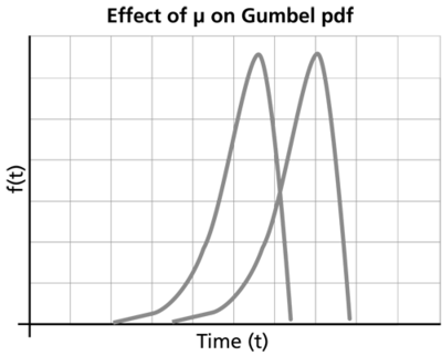
- As [math]\displaystyle{ \mu }[/math] decreases, the [math]\displaystyle{ pdf }[/math] is shifted to the left.
- As [math]\displaystyle{ \mu }[/math] increases, the [math]\displaystyle{ pdf }[/math] is shifted to the right.

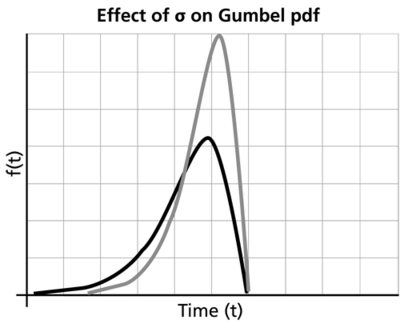
- As [math]\displaystyle{ \sigma }[/math] increases, the [math]\displaystyle{ pdf }[/math] spreads out and becomes shallower.
- As [math]\displaystyle{ \sigma }[/math] decreases, the [math]\displaystyle{ pdf }[/math] becomes taller and narrower.
- For [math]\displaystyle{ T=\pm \infty , }[/math] [math]\displaystyle{ pdf=0. }[/math] For [math]\displaystyle{ T=\mu }[/math] , the [math]\displaystyle{ pdf }[/math] reaches its maximum point [math]\displaystyle{ \frac{1}{\sigma e} }[/math]

- The points of inflection of the [math]\displaystyle{ pdf }[/math] graph are [math]\displaystyle{ T=\mu \pm \sigma \ln (\tfrac{3\pm \sqrt{5}}{2}) }[/math] or [math]\displaystyle{ T\approx \mu \pm \sigma 0.96242 }[/math] .
- If times follow the Weibull distribution, then the logarithm of times follow a Gumbel distribution. If [math]\displaystyle{ {{t}_{i}} }[/math] follows a Weibull distribution with [math]\displaystyle{ \beta }[/math] and [math]\displaystyle{ \eta }[/math] , then the [math]\displaystyle{ Ln({{t}_{i}}) }[/math] follows a Gumbel distribution with [math]\displaystyle{ \mu =\ln (\eta ) }[/math] and [math]\displaystyle{ \sigma =\tfrac{1}{\beta } }[/math] [32].