Template:Characteristics of the logistic distribution

Characteristics of the Logistic Distribution

• The logistic distribution has no shape parameter. This means that the logistic [math]\displaystyle{ pdf }[/math] has only one shape, the bell shape, and this shape does not change. The shape of the logistic distribution is very similar to that of the normal distribution.

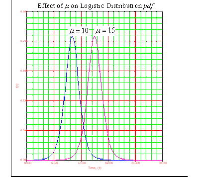
• The mean, [math]\displaystyle{ \mu }[/math] , or the mean life or the [math]\displaystyle{ MTTF }[/math] , is also the location parameter of the logistic [math]\displaystyle{ pdf }[/math] , as it locates the [math]\displaystyle{ pdf }[/math] along the abscissa. It can assume values of [math]\displaystyle{ -\infty \lt \bar{T}\lt \infty }[/math] .

• As [math]\displaystyle{ \mu }[/math] decreases, the [math]\displaystyle{ pdf }[/math] is shifted to the left.

• As [math]\displaystyle{ \mu }[/math] increases, the [math]\displaystyle{ pdf }[/math] is shifted to the right.

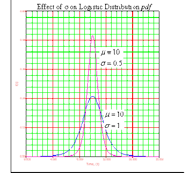
• As [math]\displaystyle{ \sigma }[/math] decreases, the [math]\displaystyle{ pdf }[/math] gets pushed toward the mean, or it becomes narrower and taller.

• As [math]\displaystyle{ \sigma }[/math] increases, the [math]\displaystyle{ pdf }[/math] spreads out away from the mean, or it becomes broader and shallower.

• The scale parameter can assume values of [math]\displaystyle{ 0\lt \sigma \lt \infty }[/math].

• The logistic [math]\displaystyle{ pdf }[/math] starts at [math]\displaystyle{ T=-\infty }[/math] with an [math]\displaystyle{ f(T)=0 }[/math] . As [math]\displaystyle{ T }[/math] increases, [math]\displaystyle{ f(T) }[/math] also increases, goes through its point of inflection and reaches its maximum value at [math]\displaystyle{ T=\bar{T} }[/math] . Thereafter, [math]\displaystyle{ f(T) }[/math] decreases, goes through its point of inflection and assumes a value of [math]\displaystyle{ f(T)=0 }[/math] at [math]\displaystyle{ T=+\infty }[/math] .

• For [math]\displaystyle{ T=\pm \infty , }[/math] the [math]\displaystyle{ pdf }[/math] equals [math]\displaystyle{ 0. }[/math] The maximum value of the [math]\displaystyle{ pdf }[/math] occurs at [math]\displaystyle{ T }[/math] = [math]\displaystyle{ \mu }[/math] and equals [math]\displaystyle{ \tfrac{1}{4\sigma }. }[/math]

• The point of inflection of the [math]\displaystyle{ pdf }[/math] plot is the point where the second derivative of the [math]\displaystyle{ pdf }[/math] equals zero. The inflection point occurs at [math]\displaystyle{ T=\mu +\sigma \ln (2\pm \sqrt{3}) }[/math] or [math]\displaystyle{ T\approx \mu \pm \sigma 1.31696 }[/math].

• If the location parameter [math]\displaystyle{ \mu }[/math] decreases, the reliability plot is shifted to the left. If [math]\displaystyle{ \mu }[/math] increases, the reliability plot is shifted to the right.

• If [math]\displaystyle{ T=\mu }[/math] then [math]\displaystyle{ R=0.5 }[/math] . is the inflection point. If [math]\displaystyle{ T\lt \mu }[/math] then [math]\displaystyle{ R(t) }[/math] is concave (concave down); if [math]\displaystyle{ T\gt \mu }[/math] then [math]\displaystyle{ R(t) }[/math] is convex (concave up). For [math]\displaystyle{ T\lt \mu , }[/math] [math]\displaystyle{ \lambda (t) }[/math] is convex (concave up), for [math]\displaystyle{ T\gt \mu ; }[/math] [math]\displaystyle{ \lambda (t) }[/math] is concave (concave down).

• The main difference between the normal distribution and logistic distribution lies in the tails and in the behavior of the failure rate function. The logistic distribution has slightly longer tails compared to the normal distribution. Also, in the upper tail of the logistic distribution, the failure rate function levels out for large [math]\displaystyle{ t }[/math] approaching 1/ [math]\displaystyle{ \delta . }[/math]

• If location parameter [math]\displaystyle{ \mu }[/math] decreases, the failure rate plot is shifted to the left. Vice versa if [math]\displaystyle{ \mu }[/math] increases, the failure rate plot is shifted to the right.

• [math]\displaystyle{ \lambda }[/math] always increases. For [math]\displaystyle{ T\to -\infty }[/math] for [math]\displaystyle{ T\to \infty }[/math] It is always [math]\displaystyle{ 0\le \lambda (t)\le \tfrac{1}{\sigma }. }[/math]

• If [math]\displaystyle{ \sigma }[/math] increases, then [math]\displaystyle{ \lambda (t) }[/math] increases more slowly and smoothly. The segment of time where [math]\displaystyle{ 0\lt \lambda (t)\lt \tfrac{1}{\sigma } }[/math] increases, too, whereas the region where [math]\displaystyle{ \lambda (t) }[/math] is close to [math]\displaystyle{ 0 }[/math] or [math]\displaystyle{ \tfrac{1}{\sigma } }[/math] gets narrower. Conversely, if [math]\displaystyle{ \sigma }[/math] decreases, then [math]\displaystyle{ \lambda (t) }[/math] increases more quickly and sharply. The segment of time where [math]\displaystyle{ 0\lt }[/math] [math]\displaystyle{ \lambda (t)\lt \tfrac{1}{\sigma } }[/math] decreases, too, whereas the region where [math]\displaystyle{ \lambda (t) }[/math] is close to [math]\displaystyle{ 0 }[/math] or [math]\displaystyle{ \tfrac{1}{\sigma } }[/math] gets broader.