Template:Confidence bounds for the gompertz model
Confidence Bounds for the Gompertz Model
The approximate reliability confidence bounds under the Gompertz model can be obtained with nonlinear regression. Additionally, the reliability is always between [math]\displaystyle{ 0 }[/math] and [math]\displaystyle{ 1 }[/math] . In order to keep the endpoints of the confidence interval, the logit transformation is used to obtain the confidence bounds on reliability.
- [math]\displaystyle{ CB=\frac{{{{\hat{R}}}_{i}}}{{{{\hat{R}}}_{i}}+(1-{{{\hat{R}}}_{i}}){{e}^{\pm {{z}_{\alpha }}{{{\hat{\sigma }}}_{R}}/\left[ {{{\hat{R}}}_{i}}(1-{{{\hat{R}}}_{i}}) \right]}}} }[/math]
- [math]\displaystyle{ {{\hat{\sigma }}^{2}}=\frac{SSE}{n-p} }[/math]
where [math]\displaystyle{ p }[/math] is the total number of groups (in this case 3) and [math]\displaystyle{ n }[/math] is the total number of items in each group.
Example 1
A device is required to have a reliability of [math]\displaystyle{ 92% }[/math] at the end of a 12-month design and development period. Table 7.1 gives the data obtained for the first five moths.
- 1) What will the reliability be at the end of this 12-month period?
- 2) What will the maximum achievable reliability be if the reliability program plan pursued during the first 5 months is continued?
- 3) How do the predicted reliability values compare with the actual values?
Solution
Having completed Steps 1 through 4 by preparing Table 7.1 and calculating the last column of the table to find [math]\displaystyle{ {{S}_{1}} }[/math] , [math]\displaystyle{ {{S}_{2}} }[/math] and [math]\displaystyle{ {{S}_{3}} }[/math] , proceed as follows:
- a) Find [math]\displaystyle{ c }[/math] from Eqn. (eq9).
- [math]\displaystyle{ \begin{align} & c= & {{\left( \frac{8.850-8.641}{8.641-8.250} \right)}^{\tfrac{1}{2}}} \\ & = & 0.731 \end{align} }[/math]
- b) Find [math]\displaystyle{ a }[/math] from Eqn. (eq10).
- This is the upper limit for the reliability as [math]\displaystyle{ T\to \infty }[/math] .
- c) Find [math]\displaystyle{ b }[/math] from Eqn. (eq11).
- [math]\displaystyle{ \begin{align} & b= & {{e}^{\left[ \tfrac{(8.641-8.250)(0.731-1)}{{{(1-{{0.731}^{2}})}^{2}}} \right]}} \\ & = & {{e}^{(-0.485)}} \\ & = & 0.615 \end{align} }[/math]
- Now, since the initial values have been determined, the Gauss-Newton method can be used. Therefore, substituting [math]\displaystyle{ {{Y}_{i}}={{R}_{i}}, }[/math] [math]\displaystyle{ g_{1}^{(0)}=94.16, }[/math] [math]\displaystyle{ g_{2}^{(0)}=0.615, }[/math] [math]\displaystyle{ g_{3}^{(0)}=0.731, }[/math] [math]\displaystyle{ {{Y}^{(0)}},{{D}^{(0)}}, }[/math] [math]\displaystyle{ {{\nu }^{(0)}} }[/math] become:
- [math]\displaystyle{ {{Y}^{(0)}}=\left[ \begin{matrix} 0.0916 \\ 0.0015 \\ -0.1190 \\ 0.1250 \\ 0.0439 \\ -0.0743 \\ \end{matrix} \right] }[/math]
- [math]\displaystyle{ {{D}^{(0)}}=\left[ \begin{matrix} 0.6150 & 94.1600 & 0.0000 \\ 0.7009 & 78.4470 & -32.0841 \\ 0.7712 & 63.0971 & -51.6122 \\ 0.8270 & 49.4623 & -60.6888 \\ 0.8704 & 38.0519 & -62.2513 \\ 0.9035 & 28.8742 & -59.0463 \\ \end{matrix} \right] }[/math]
- [math]\displaystyle{ {{\nu }^{(0)}}=\left[ \begin{matrix} g_{1}^{(0)} \\ g_{2}^{(0)} \\ g_{3}^{(0)} \\ \end{matrix} \right]=\left[ \begin{matrix} 94.16 \\ 0.615 \\ 0.731 \\ \end{matrix} \right] }[/math]
The estimate of the parameters [math]\displaystyle{ {{\nu }^{(0)}} }[/math] is given by:
The revised estimated regression coefficients in matrix form are:
- [math]\displaystyle{ {{Q}^{(k+1)}}\lt {{Q}^{(k)}} }[/math]
If the Gauss-Newton method works effectively, then the relationship has to hold, meaning that [math]\displaystyle{ {{g}^{(k+1)}} }[/math] gives better estimates than [math]\displaystyle{ {{g}^{(k)}} }[/math] , after [math]\displaystyle{ k }[/math] . With the starting coefficients, [math]\displaystyle{ {{g}^{(0)}}, }[/math] [math]\displaystyle{ Q }[/math] is:
And with the coefficients at the end of the first iteration, [math]\displaystyle{ {{g}^{(1)}}, }[/math] [math]\displaystyle{ Q }[/math] is:
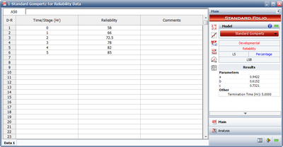
Therefore, it can be justified that the Gauss-Newton method works in the right direction. The iterations are continued until the relationship of Eqn.(crit) is satisfied. Note that RGA uses a different analysis method called the Levenberg-Marquardt. This method utilizes the best features of the Gauss-Newton method and the method of the steepest descent, and occupies a middle ground between these two methods. The estimated parameters using RGA are shown in Figure SGomp1. They are:
- [math]\displaystyle{ \begin{align} & \widehat{a}= & 0.9422 \\ & \widehat{b}= & 0.6152 \\ & \widehat{c}= & 0.7321 \end{align} }[/math]
The Gompertz reliability growth curve is:
- [math]\displaystyle{ R=0.9422{{(0.6152)}^{{{0.7321}^{T}}}} }[/math]
- 1) The achievable reliability at the end of the 12-month period of design and development is:
The required reliability is [math]\displaystyle{ 92% }[/math] . Consequently, from the previous result, this requirement will barely be met. Every effort should therefore be expended to implement the reliability program plan fully, and perhaps augment it slightly to assure that the reliability goal will be met.
- 2) The maximum achievable reliability from Step 2, or from the value of [math]\displaystyle{ a }[/math] , is [math]\displaystyle{ 0.9422 }[/math] .
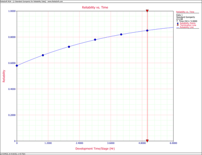
- 3) The predicted reliability values, as calculated from the Gompertz equation, Eqn. (eq8), are compared with the actual data in Table 7.2. It may be seen in Table 7.2 that the Gompertz curve appears to provide a very good fit for the data used, since the equation reproduces the available data with less than [math]\displaystyle{ 1% }[/math] error. Eqn. (eq8) is plotted in Figure oldfig32 and identifies the type of reliability growth curve this equation represents.
| Growth Time [math]\displaystyle{ T }[/math](months) | Gompertz Reliability(%) | Raw Data Reliability(%) |
|---|---|---|
| 0 | 57.97 | 58.00 |
| 1 | 66.02 | 66.00 |
| 2 | 72.62 | 72.50 |
| 3 | 77.87 | 78.00 |
| 4 | 81.95 | 82.00 |
| 5 | 85.07 | 85.00 |
| 6 | 87.43 | |
| 7 | 89.20 | |
| 8 | 90.52 | |
| 9 | 91.50 | |
| 10 | 92.22 | |
| 11 | 92.75 | |
| 12 | 93.14 |
Example 2
Calculate the parameters of the Gompertz model using the sequential data in Table 7.3.
| Run Number | Result | Successes | Observed Reliability(%) |
|---|---|---|---|
| 1 | F | 0 | |
| 2 | F | 0 | |
| 3 | F | 0 | |
| 4 | S | 1 | 25.00 |
| 5 | F | 1 | 20.00 |
| 6 | F | 1 | 16.67 |
| 7 | S | 2 | 28.57 |
| 8 | S | 3 | 37.50 |
| 9 | S | 4 | 44.44 |
| 10 | S | 5 | 50.00 |
| 11 | S | 6 | 54.55 |
| 12 | S | 7 | 58.33 |
| 13 | S | 8 | 61.54 |
| 14 | S | 9 | 64.29 |
| 15 | S | 10 | 66.67 |
| 16 | S | 11 | 68.75 |
| 17 | F | 11 | 64.71 |
| 18 | S | 12 | 66.67 |
| 19 | F | 12 | 63.16 |
| 20 | S | 13 | 65.00 |
| 21 | S | 14 | 66.67 |
| 22 | S | 15 | 68.18 |
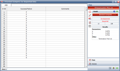
Solution Using RGA, the parameter estimates are shown in Figure SGomp2.


