Template:Example: 2P Weibull Distribution RRY: Difference between revisions
No edit summary |
Kate Racaza (talk | contribs) No edit summary |
||
| Line 37: | Line 37: | ||
Utilizing the values from | Utilizing the values from the table, calculate <math> \hat{a} </math> and <math> \hat{b} </math> using the following equations: | ||
::<math> \hat{b} =\frac{\sum\limits_{i=1}^{6}(\ln t_{i})y_{i}-(\sum\limits_{i=1}^{6}\ln t_{i})(\sum\limits_{i=1}^{6}y_{i})/6}{ \sum\limits_{i=1}^{6}(\ln t_{i})^{2}-(\sum\limits_{i=1}^{6}\ln t_{i})^{2}/6} | ::<math> \hat{b} =\frac{\sum\limits_{i=1}^{6}(\ln t_{i})y_{i}-(\sum\limits_{i=1}^{6}\ln t_{i})(\sum\limits_{i=1}^{6}y_{i})/6}{ \sum\limits_{i=1}^{6}(\ln t_{i})^{2}-(\sum\limits_{i=1}^{6}\ln t_{i})^{2}/6} | ||
</math> | </math> | ||
| Line 70: | Line 70: | ||
::<math> \hat{\rho }=0.9956 </math> | ::<math> \hat{\rho }=0.9956 </math> | ||
<br> | <br> | ||
This example can be repeated in the Weibull++ software, as shown next. The following picture shows a Weibull++ standard folio data sheet calculated with the 2P-Weibull distribution and rank regression on Y. | |||
[[Image:Weibull Distribution Example 3 RRY Result.png|thumb|center|400px| ]] | [[Image:Weibull Distribution Example 3 RRY Result.png|thumb|center|400px| ]] | ||
The following plot shows the Weibull probability plot for the data set (with 90% two-sided confidence bounds). | |||
The plot | |||
[[Image:Weibull Distribution Example 3 RRY Confidence Plot.png|thumb|center|400px| ]] | [[Image:Weibull Distribution Example 3 RRY Confidence Plot.png|thumb|center|400px| ]] | ||
If desired, the Weibull <math>pdf</math> representing | If desired, the Weibull <math>pdf</math> representing the data set can be written as: | ||
::<math> f(t)={\frac{\beta }{\eta }}\left( {\frac{t}{\eta }}\right) ^{\beta -1}e^{-\left( {\frac{t}{\eta }}\right) ^{\beta }} </math> | ::<math> f(t)={\frac{\beta }{\eta }}\left( {\frac{t}{\eta }}\right) ^{\beta -1}e^{-\left( {\frac{t}{\eta }}\right) ^{\beta }} </math> | ||
| Line 127: | Line 88: | ||
::<math> f(t)={\frac{1.4302}{76.317}}\left( {\frac{t}{76.317}}\right) ^{0.4302}e^{-\left( {\frac{t}{76.317}}\right) ^{1.4302}} </math> | ::<math> f(t)={\frac{1.4302}{76.317}}\left( {\frac{t}{76.317}}\right) ^{0.4302}e^{-\left( {\frac{t}{76.317}}\right) ^{1.4302}} </math> | ||
You can also plot | You can also plot this result by selecting '''Pdf Plot''' on the Plot Type drop-down list on the control panel. | ||
[[Image:Weibull Distribution Example 3 pdf Plot.png|thumb|center|400px]] | [[Image:Weibull Distribution Example 3 pdf Plot.png|thumb|center|400px]] | ||
From this point on, different results, reports and plots can be obtained. | From this point on, different results, reports and plots can be obtained. | ||
Revision as of 23:24, 6 April 2012
2P Weibull Distribution RRY Example
Consider the data in Example 1, where six units were tested to failure and the following failure times were recorded: 16, 34, 53, 75, 93 and 120 hours. Estimate the parameters and the correlation coefficient using rank regression on Y, assuming that the data follow the two-parameter Weibull distribution.
Solution
Construct a table as shown below.
| Table - Least Squares Analysis | |||||||
| [math]\displaystyle{ N }[/math] | [math]\displaystyle{ T_{i} }[/math] | [math]\displaystyle{ ln(T_{i}) }[/math] | [math]\displaystyle{ F(T_i) }[/math] | [math]\displaystyle{ y_{i} }[/math] | [math]\displaystyle{ (ln{T_i})^2 }[/math] | [math]\displaystyle{ {y_i}^2 }[/math] | [math]\displaystyle{ (ln{T_i})y_i }[/math] |
|---|---|---|---|---|---|---|---|
| 1 | 16 | 2.7726 | 0.1091 | -2.1583 | 7.6873 | 4.6582 | -5.9840 |
| 2 | 34 | 3.5264 | 0.2645 | -1.1802 | 12.4352 | 1.393 | -4.1620 |
| 3 | 53 | 3.9703 | 0.4214 | -0.6030 | 15.7632 | 0.3637 | -2.3943 |
| 4 | 75 | 4.3175 | 0.5786 | -0.146 | 18.6407 | 0.0213 | -0.6303 |
| 5 | 93 | 4.5326 | 0.7355 | 0.2851 | 20.5445 | 0.0813 | 1.2923 |
| 6 | 120 | 4.7875 | 0.8909 | 0.7955 | 22.9201 | 0.6328 | 3.8083 |
| [math]\displaystyle{ \sum }[/math] | 23.9068 | -3.007 | 97.9909 | 7.1502 | -8.0699 | ||
Utilizing the values from the table, calculate [math]\displaystyle{ \hat{a} }[/math] and [math]\displaystyle{ \hat{b} }[/math] using the following equations:
- [math]\displaystyle{ \hat{b} =\frac{\sum\limits_{i=1}^{6}(\ln t_{i})y_{i}-(\sum\limits_{i=1}^{6}\ln t_{i})(\sum\limits_{i=1}^{6}y_{i})/6}{ \sum\limits_{i=1}^{6}(\ln t_{i})^{2}-(\sum\limits_{i=1}^{6}\ln t_{i})^{2}/6} }[/math]
- [math]\displaystyle{ \hat{b}=\frac{-8.0699-(23.9068)(-3.0070)/6}{97.9909-(23.9068)^{2}/6} }[/math]
or
- [math]\displaystyle{ \hat{b}=1.4301 }[/math]
and:
- [math]\displaystyle{ \hat{a}=\overline{y}-\hat{b}\overline{T}=\frac{\sum \limits_{i=1}^{N}y_{i}}{N}-\hat{b}\frac{\sum\limits_{i=1}^{N}\ln t_{i}}{N } }[/math]
or:
- [math]\displaystyle{ \hat{a}=\frac{(-3.0070)}{6}-(1.4301)\frac{23.9068}{6}=-6.19935 }[/math]
Therefore:
- [math]\displaystyle{ \hat{\beta }=\hat{b}=1.4301 }[/math]
and:
- [math]\displaystyle{ \hat{\eta }=e^{-\frac{\hat{a}}{\hat{b}}}=e^{-\frac{(-6.19935)}{ 1.4301}} }[/math]
or:
- [math]\displaystyle{ \hat{\eta }=76.318\text{ hr} }[/math]
The correlation coefficient can be estimated as:
- [math]\displaystyle{ \hat{\rho }=0.9956 }[/math]
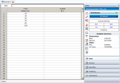
This example can be repeated in the Weibull++ software, as shown next. The following picture shows a Weibull++ standard folio data sheet calculated with the 2P-Weibull distribution and rank regression on Y.
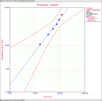
The following plot shows the Weibull probability plot for the data set (with 90% two-sided confidence bounds).
If desired, the Weibull [math]\displaystyle{ pdf }[/math] representing the data set can be written as:
- [math]\displaystyle{ f(t)={\frac{\beta }{\eta }}\left( {\frac{t}{\eta }}\right) ^{\beta -1}e^{-\left( {\frac{t}{\eta }}\right) ^{\beta }} }[/math]
or:
- [math]\displaystyle{ f(t)={\frac{1.4302}{76.317}}\left( {\frac{t}{76.317}}\right) ^{0.4302}e^{-\left( {\frac{t}{76.317}}\right) ^{1.4302}} }[/math]
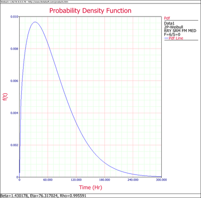
You can also plot this result by selecting Pdf Plot on the Plot Type drop-down list on the control panel.
From this point on, different results, reports and plots can be obtained.


