Template:Example: Bayesian Test Design with Prior Information from Expert Opinion

Bayesian Test Design with Prior Information from Expert Opinion

Suppose you wanted to know the reliability of a system and you had the following prior knowledge of the system:

• Lowest possible reliability: a = 0.8

• Most likely reliability: b = 0.85

• Highest possible reliability: c = 0.97

This information can be used to approximate the expected value and the variance of the prior system reliability.

[math]\displaystyle{ E\left(R_{0}\right)=\frac{a+4b+c}{6}=0.861667 }[/math]

[math]\displaystyle{ Var\left(R_{0}\right)=\frac{c-a}{6}=0.028333 }[/math]

These approximations of the expected value and variance of the prior system reliability can then be used to estimate [math]\displaystyle{ \alpha_{0} }[/math] and [math]\displaystyle{ \beta_{0} }[/math] used in the Beta distribution for the system reliability, as given next:

[math]\displaystyle{ \alpha\,\!_{0}=E\left(R_{0}\right)\left[\frac{E\left(R_{0}\right)-E^{2}\left(R_{0}\right)}{Var\left(R_{0}\right)}-1\right]=2.763331 }[/math]

[math]\displaystyle{ \beta\,\!_{0}=\left(1-E\left(R_{0}\right)\right)\left[\frac{E\left(R_{0}\right)-E^{2}\left(R_{0}\right)}{Var\left(R_{0}\right)}-1\right]=0.44363 }[/math]

With [math]\displaystyle{ \alpha_{0} }[/math] and [math]\displaystyle{ \beta_{0} }[/math] known, any single value of the 4 quantities system reliability R, confidence level CL, number of units n, or number of failures r can be calculated from the other 3 using the Beta distribution function:

[math]\displaystyle{ 1-CL=\text{Beta}\left(R,\alpha,\beta\right)=\text{Beta}\left(R,n-r+\alpha_{0},r+\beta_{0}\right) }[/math]

Solve for System Reliability R

Given CL = 0.8, n = 20, and r = 1, using the above prior information to solve R.

First, we get the number of successes s is:

[math]\displaystyle{ s = n – r = 19 }[/math]

Then the parameters in the posterior Beta distribution for R are calculated as:

[math]\displaystyle{ \alpha\,\!=\alpha\,\!_{0}+s=21.76333 }[/math]

[math]\displaystyle{ \beta\,\!=\beta\,\!_{0}+r=1.44363 }[/math]

Finally, from this posterior distribution,the system reliability R at confidence level of CL=0.8 is solved as:

[math]\displaystyle{ R=\text{BetaINV}\left(1-CL,\alpha\,\!,\beta\,\!\right)=0.902996 }[/math]

Solve for Confidence Level CL

Given R = 0.9, n = 20, and r = 1, using the above prior information on system reliability to solve for CL.

First, we get the number of successes s is:

[math]\displaystyle{ s = n – r = 19 }[/math]

Then the parameters in the posterior Beta distribution for R are calculated as:

[math]\displaystyle{ \alpha\,\!=\alpha\,\!_{0}+s=21.76333 }[/math]

[math]\displaystyle{ \beta\,\!=\beta\,\!_{0}+r=1.44363 }[/math]

Finally, from this posterior distribution, the corresponding confidence level for reliability R=0.9 is:

[math]\displaystyle{ CL=\text{Beta}\left(R,\alpha,\beta\right)=0.812164 }[/math]

Solve for Sample Size n

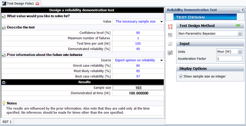
Given R = 0.9, CL = 0.8, and r = 1, using the above prior information on system reliability to solve the required sample size in the demonstration test.

Again the above Beta distribution equation for the system reliability can be utilized. The figure in below shows the result from Weibull++.

The above results shows the required sample size is 20. Weibull++ always displays the sample size as an integer.