Template:Example: Likelihood Ratio Bounds on Reliability (Type 2): Difference between revisions
No edit summary |
No edit summary |
||
| (7 intermediate revisions by 4 users not shown) | |||
| Line 1: | Line 1: | ||
'''Likelihood Ratio Bounds on Reliability (Type 2)''' | '''Likelihood Ratio Bounds on Reliability (Type 2)''' | ||
For the data given in Example 1, determine the 90% two-sided confidence bounds on the reliability estimate for <math>t=45</math>. The ML estimate for the reliability at <math>t=45</math> is 14.816%. | For the data given in Example 1, determine the 90% two-sided confidence bounds on the reliability estimate for <math>t=45\,\!</math>. The ML estimate for the reliability at <math>t=45\,\!</math> is 14.816%. | ||
'''Solution''' | '''Solution''' | ||
In this example, we are trying to determine the 90% two-sided confidence bounds on the reliability estimate of 14.816%. As was mentioned, we need to rewrite the likelihood ratio equation so that it is in terms of <math>R</math> and <math>\beta .</math> This is again accomplished by substituting the Weibull reliability equation into the <math>\eta </math> term in the likelihood ratio equation to form a likelihood equation in terms of <math>R</math> and <math>\beta </math>: | In this example, we are trying to determine the 90% two-sided confidence bounds on the reliability estimate of 14.816%. As was mentioned, we need to rewrite the likelihood ratio equation so that it is in terms of <math>R\,\!</math> and <math>\beta .\,\!</math> This is again accomplished by substituting the Weibull reliability equation into the <math>\eta \,\!</math> term in the likelihood ratio equation to form a likelihood equation in terms of <math>R\,\!</math> and <math>\beta \,\!</math>: | ||
::<math>\begin{align} | ::<math>\begin{align} | ||
& L(\beta ,R)= & \underset{i=1}{\overset{N}{\mathop \prod }}\,f({{x}_{i}};\beta ,t,R) \\ | & L(\beta ,R)= & \underset{i=1}{\overset{N}{\mathop \prod }}\,f({{x}_{i}};\beta ,t,R) \\ | ||
& & | & & | ||
\end{align}</math> | \end{align}\,\!</math> | ||
::<math>=\underset{i=1}{\overset{5}{\mathop \prod }}\,\frac{\beta }{\left( \tfrac{t}{{{(-\text{ln}(R))}^{\tfrac{1}{\beta }}}} \right)}\cdot {{\left( \frac{{{x}_{i}}}{\left( \tfrac{t}{{{(-\text{ln}(R))}^{\tfrac{1}{\beta }}}} \right)} \right)}^{\beta -1}}\cdot \text{exp}\left[ -{{\left( \frac{{{x}_{i}}}{\left( \tfrac{t}{{{(-\text{ln}(R))}^{\tfrac{1}{\beta }}}} \right)} \right)}^{\beta }} \right]</math> | ::<math>=\underset{i=1}{\overset{5}{\mathop \prod }}\,\frac{\beta }{\left( \tfrac{t}{{{(-\text{ln}(R))}^{\tfrac{1}{\beta }}}} \right)}\cdot {{\left( \frac{{{x}_{i}}}{\left( \tfrac{t}{{{(-\text{ln}(R))}^{\tfrac{1}{\beta }}}} \right)} \right)}^{\beta -1}}\cdot \text{exp}\left[ -{{\left( \frac{{{x}_{i}}}{\left( \tfrac{t}{{{(-\text{ln}(R))}^{\tfrac{1}{\beta }}}} \right)} \right)}^{\beta }} \right]\,\!</math> | ||
where <math>{{x}_{i}}\,\!</math> are the original time-to-failure data points. We can now rearrange the likelihood ratio equation to the form: | |||
::<math>L(\beta ,R)-L(\widehat{\beta },\widehat{\eta })\cdot {{e}^{\tfrac{-\chi _{\alpha ;1}^{2}}{2}}}=0\,\!</math> | |||
Since our specified confidence level, <math>\delta \,\!</math>, is 90%, we can calculate the value of the chi-squared statistic, <math>\chi _{0.9;1}^{2}=2.705543.\,\!</math> We can now substitute this information into the equation: | |||
Since our specified confidence level, <math>\delta </math>, is 90%, we can calculate the value of the chi-squared statistic, <math>\chi _{0.9;1}^{2}=2.705543.</math> We can now substitute this information into the equation: | |||
::<math>\begin{align} | ::<math>\begin{align} | ||
| Line 28: | Line 26: | ||
\\ | \\ | ||
L(\beta ,R)-4.432926\cdot {{10}^{-10}}= & 0 | L(\beta ,R)-4.432926\cdot {{10}^{-10}}= & 0 | ||
\end{align} | \end{align}\,\!</math> | ||
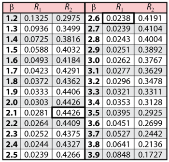
It now remains to find the values of <math>\beta \,\!</math> and <math>R\,\!</math> that satisfy this equation. This is an iterative process that requires setting the value of <math>\beta \,\!</math> and finding the appropriate values of <math>R\,\!</math>. The following table gives the values of <math>R\,\!</math> based on given values of <math>\beta \,\!</math>. | |||
[[Image:confidencechart3.png|center|350px|]] | |||
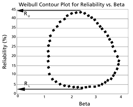
These points are represented graphically in the following contour plot: | These points are represented graphically in the following contour plot: | ||
[[Image:weibull contour plot reliability beta.png|center|425px|]] | |||
As can be determined from the table, the lowest calculated value for <math>R\,\!</math> is 2.38%, while the highest is 44.26%. These represent the 90% two-sided confidence limits on the reliability at <math>t=45\,\!</math>. | |||
As can be determined from the table, the lowest calculated value for <math>R</math> is 2.38%, while the highest is 44.26%. These represent the 90% two-sided confidence limits on the reliability at <math>t=45</math>. | |||
Latest revision as of 17:54, 21 December 2015
Likelihood Ratio Bounds on Reliability (Type 2)
For the data given in Example 1, determine the 90% two-sided confidence bounds on the reliability estimate for [math]\displaystyle{ t=45\,\! }[/math]. The ML estimate for the reliability at [math]\displaystyle{ t=45\,\! }[/math] is 14.816%.
Solution
In this example, we are trying to determine the 90% two-sided confidence bounds on the reliability estimate of 14.816%. As was mentioned, we need to rewrite the likelihood ratio equation so that it is in terms of [math]\displaystyle{ R\,\! }[/math] and [math]\displaystyle{ \beta .\,\! }[/math] This is again accomplished by substituting the Weibull reliability equation into the [math]\displaystyle{ \eta \,\! }[/math] term in the likelihood ratio equation to form a likelihood equation in terms of [math]\displaystyle{ R\,\! }[/math] and [math]\displaystyle{ \beta \,\! }[/math]:
- [math]\displaystyle{ \begin{align} & L(\beta ,R)= & \underset{i=1}{\overset{N}{\mathop \prod }}\,f({{x}_{i}};\beta ,t,R) \\ & & \end{align}\,\! }[/math]
- [math]\displaystyle{ =\underset{i=1}{\overset{5}{\mathop \prod }}\,\frac{\beta }{\left( \tfrac{t}{{{(-\text{ln}(R))}^{\tfrac{1}{\beta }}}} \right)}\cdot {{\left( \frac{{{x}_{i}}}{\left( \tfrac{t}{{{(-\text{ln}(R))}^{\tfrac{1}{\beta }}}} \right)} \right)}^{\beta -1}}\cdot \text{exp}\left[ -{{\left( \frac{{{x}_{i}}}{\left( \tfrac{t}{{{(-\text{ln}(R))}^{\tfrac{1}{\beta }}}} \right)} \right)}^{\beta }} \right]\,\! }[/math]
where [math]\displaystyle{ {{x}_{i}}\,\! }[/math] are the original time-to-failure data points. We can now rearrange the likelihood ratio equation to the form:
- [math]\displaystyle{ L(\beta ,R)-L(\widehat{\beta },\widehat{\eta })\cdot {{e}^{\tfrac{-\chi _{\alpha ;1}^{2}}{2}}}=0\,\! }[/math]
Since our specified confidence level, [math]\displaystyle{ \delta \,\! }[/math], is 90%, we can calculate the value of the chi-squared statistic, [math]\displaystyle{ \chi _{0.9;1}^{2}=2.705543.\,\! }[/math] We can now substitute this information into the equation:
- [math]\displaystyle{ \begin{align} L(\beta ,R)-L(\widehat{\beta },\widehat{\eta })\cdot {{e}^{\tfrac{-\chi _{\alpha ;1}^{2}}{2}}}= & 0 \\ \\ L(\beta ,R)-1.714714\times {{10}^{-9}}\cdot {{e}^{\tfrac{-2.705543}{2}}}= & 0 \\ \\ L(\beta ,R)-4.432926\cdot {{10}^{-10}}= & 0 \end{align}\,\! }[/math]
It now remains to find the values of [math]\displaystyle{ \beta \,\! }[/math] and [math]\displaystyle{ R\,\! }[/math] that satisfy this equation. This is an iterative process that requires setting the value of [math]\displaystyle{ \beta \,\! }[/math] and finding the appropriate values of [math]\displaystyle{ R\,\! }[/math]. The following table gives the values of [math]\displaystyle{ R\,\! }[/math] based on given values of [math]\displaystyle{ \beta \,\! }[/math].
These points are represented graphically in the following contour plot:
As can be determined from the table, the lowest calculated value for [math]\displaystyle{ R\,\! }[/math] is 2.38%, while the highest is 44.26%. These represent the 90% two-sided confidence limits on the reliability at [math]\displaystyle{ t=45\,\! }[/math].

