Template:Example: Lognormal Distribution Likelihood Ratio Bound (Time): Difference between revisions
(Created page with ''''Lognormal Distribution Likelihood Ratio Bound Example (Time)''' For the data given in Example 5, determine the two-sided 75% confidence bounds on the time estimate for a reli…') |
No edit summary |
||
| Line 1: | Line 1: | ||
'''Lognormal Distribution Likelihood Ratio Bound Example (Time)''' | '''Lognormal Distribution Likelihood Ratio Bound Example (Time)''' | ||
For the data given in Example 5, determine the two-sided 75% confidence bounds on the time estimate for a reliability of 80%. The ML estimate for the time at <math>R(t)=80%</math> is 55.718. | For the data given in [[Lognormal Example 5 Data|Example 5]], determine the two-sided 75% confidence bounds on the time estimate for a reliability of 80%. The ML estimate for the time at <math>R(t)=80%</math> is 55.718. | ||
'''Solution''' | '''Solution''' | ||
Revision as of 23:24, 13 February 2012
Lognormal Distribution Likelihood Ratio Bound Example (Time)
For the data given in Example 5, determine the two-sided 75% confidence bounds on the time estimate for a reliability of 80%. The ML estimate for the time at [math]\displaystyle{ R(t)=80% }[/math] is 55.718.
Solution
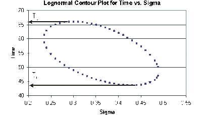
In this example, we are trying to determine the two-sided 75% confidence bounds on the time estimate of 55.718. This is accomplished by substituting [math]\displaystyle{ R=0.80 }[/math] and [math]\displaystyle{ \alpha =0.75 }[/math] into Eqn. (lognormliketr), and varying [math]\displaystyle{ {{\sigma }_{{{T}'}}} }[/math] until the maximum and minimum values of [math]\displaystyle{ t }[/math] are found. The following table gives the values of [math]\displaystyle{ t }[/math] based on given values of [math]\displaystyle{ {{\sigma }_{{{T}'}}} }[/math] .
This data set is represented graphically in the following contour plot:
As can be determined from the table, the lowest calculated value for [math]\displaystyle{ t }[/math] is 43.634, while the highest is 66.085. These represent the two-sided 75% confidence limits on the time at which reliability is equal to 80%.
