Template:Example: Lognormal Distribution Probability Plot

Lognormal Distribution Probability Plotting Example

Eight units are put on a life test and tested to failure. The failures occurred at 45, 140, 260, 500, 850, 1400, 3000, and 9000 hours. Estimate the parameters for the lognormal distribution using probability plotting.

Solution

In order to plot the points for the probability plot, the appropriate unreliability estimate values must be obtained. These will be estimated through the use of median ranks, which can be obtained from statistical tables or the Quick Statistical Reference in Weibull++. The following table shows the times-to-failure and the appropriate median rank values for this example:

[math]\displaystyle{ \begin{matrix} \text{Time-to-} & \text{Median} \\ \text{Failure (hr}\text{.)} & \text{Rank ( }\!\!%\!\!\text{ )} \\ \text{ 45} & \text{ 8}\text{.30 }\!\!%\!\!\text{ } \\ \text{ 140} & \text{20}\text{.11 }\!\!%\!\!\text{ } \\ \text{ 260} & \text{32}\text{.05 }\!\!%\!\!\text{ } \\ \text{ 500} & \text{44}\text{.02 }\!\!%\!\!\text{ } \\ \text{ 850} & \text{55}\text{.98 }\!\!%\!\!\text{ } \\ \text{1400} & \text{67}\text{.95 }\!\!%\!\!\text{ } \\ \text{3000} & \text{79}\text{.89 }\!\!%\!\!\text{ } \\ \text{9000} & \text{91}\text{.70 }\!\!%\!\!\text{ } \\ \end{matrix} }[/math]

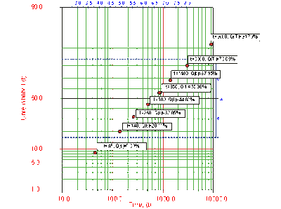
These points may now be plotted on normal probability plotting paper as shown in the next figure.

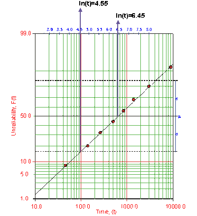
Draw the best possible line through the plot points. The time values where this line intersects the 15.85% and 50% unreliability values should be projected up to the logarithmic scale, as shown in the following plot.

The natural logarithm of the time where the fitted line intersects .. is equivalent to [math]\displaystyle{ {\mu }' }[/math] . In this case, [math]\displaystyle{ {\mu }'=6.45 }[/math] . The value for [math]\displaystyle{ {{\sigma }_{{{T}'}}} }[/math] is equal to the difference between the natural logarithms of the times where the fitted line crosses [math]\displaystyle{ Q(t)=50% }[/math] and [math]\displaystyle{ Q(t)=15.85%. }[/math] At [math]\displaystyle{ Q(t)=15.85% }[/math] , ln [math]\displaystyle{ (t)=4.55 }[/math] . Therefore, [math]\displaystyle{ {\sigma'}=6.45-4.55=1.9 }[/math] .