Template:Example: Normal Distribution Likelihood Ratio Bound (Parameters): Difference between revisions
No edit summary |
Nikki Helms (talk | contribs) No edit summary |
||
| Line 33: | Line 33: | ||
The following table gives the values of <math>\sigma </math> based on given values of <math>\mu </math> . | The following table gives the values of <math>\sigma </math> based on given values of <math>\mu </math> . | ||
[[Image:tableofmu. | [[Image:tableofmu.png|center|400px| ]] | ||
<math></math> | <math></math> | ||
Revision as of 21:57, 2 April 2012
Normal Distribution Likelihood Ratio Bound Example (Parameters)
Five units are put on a reliability test and experience failures at 12, 24, 28, 34, and 46 hours. Assuming a normal distribution, the MLE parameter estimates are calculated to be [math]\displaystyle{ \widehat{\mu }=28.8 }[/math] and [math]\displaystyle{ \widehat{\sigma }=11.2143. }[/math] Calculate the two-sided 80% confidence bounds on these parameters using the likelihood ratio method.
Solution
The first step is to calculate the likelihood function for the parameter estimates:
- [math]\displaystyle{ \begin{align} L(\widehat{\mu },\widehat{\sigma })= & \underset{i=1}{\overset{N}{\mathop \prod }}\,f({{t}_{i}};\widehat{\mu },\widehat{\sigma })=\underset{i=1}{\overset{5}{\mathop \prod }}\,\frac{1}{\widehat{\sigma }\cdot \sqrt{2\pi }}\cdot {{e}^{-\tfrac{1}{2}{{\left( \tfrac{{{t}_{i}}-\widehat{\mu }}{\widehat{\sigma }} \right)}^{2}}}} \\ L(\widehat{\mu },\widehat{\sigma })= & \underset{i=1}{\overset{5}{\mathop \prod }}\,\frac{1}{11.2143\cdot \sqrt{2\pi }}\cdot {{e}^{-\tfrac{1}{2}{{\left( \tfrac{{{t}_{i}}-28.8}{11.2143} \right)}^{2}}}} \\ L(\widehat{\mu },\widehat{\sigma })= & 4.676897\times {{10}^{-9}} \end{align} }[/math]
where [math]\displaystyle{ {{t}_{i}} }[/math] are the original time-to-failure data points. We can now rearrange the likelihood ratio equation to the form:
- [math]\displaystyle{ L(\mu ,\sigma )-L(\widehat{\mu },\widehat{\sigma })\cdot {{e}^{\tfrac{-\chi _{\alpha ;1}^{2}}{2}}}=0 }[/math]
Since our specified confidence level, [math]\displaystyle{ \delta }[/math] , is 80%, we can calculate the value of the chi-squared statistic, [math]\displaystyle{ \chi _{0.8;1}^{2}=1.642374. }[/math] We can now substitute this information into the equation:
- [math]\displaystyle{ \begin{align} L(\mu ,\sigma )-L(\widehat{\mu },\widehat{\sigma })\cdot {{e}^{\tfrac{-\chi _{\alpha ;1}^{2}}{2}}}= & 0, \\ \\ L(\mu ,\sigma )-4.676897\times {{10}^{-9}}\cdot {{e}^{\tfrac{-1.642374}{2}}}= & 0, \\ \\ L(\mu ,\sigma )-2.057410\times {{10}^{-9}}= & 0. \end{align} }[/math]
It now remains to find the values of [math]\displaystyle{ \mu }[/math] and [math]\displaystyle{ \sigma }[/math] which satisfy this equation. This is an iterative process that requires setting the value of [math]\displaystyle{ \mu }[/math] and finding the appropriate values of [math]\displaystyle{ \sigma }[/math] , and vice versa.
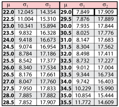
The following table gives the values of [math]\displaystyle{ \sigma }[/math] based on given values of [math]\displaystyle{ \mu }[/math] .
[math]\displaystyle{ }[/math]
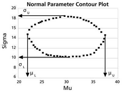
This data set is represented graphically in the following contour plot:
(Note that this plot is generated with degrees of freedom [math]\displaystyle{ k=1 }[/math] , as we are only determining bounds on one parameter. The contour plots generated in Weibull++ are done with degrees of freedom [math]\displaystyle{ k=2 }[/math] , for use in comparing both parameters simultaneously.) As can be determined from the table, the lowest calculated value for [math]\displaystyle{ \sigma }[/math] is 7.849, while the highest is 17.909. These represent the two-sided 80% confidence limits on this parameter. Since solutions for the equation do not exist for values of [math]\displaystyle{ \mu }[/math] below 22 or above 35.5, these can be considered the two-sided 80% confidence limits for this parameter. In order to obtain more accurate values for the confidence limits on [math]\displaystyle{ \mu }[/math] , we can perform the same procedure as before, but finding the two values of [math]\displaystyle{ \mu }[/math] that correspond with a given value of [math]\displaystyle{ \sigma . }[/math] Using this method, we find that the two-sided 80% confidence limits on [math]\displaystyle{ \mu }[/math] are 21.807 and 35.793, which are close to the initial estimates of 22 and 35.5.

