Template:Example: Normal Distribution MLE
Normal Distribution MLE Example
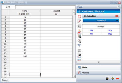
Using the data of Example 2 and assuming a normal distribution, estimate the parameters using the MLE method.
Solution
In this example we have non-grouped data without suspensions and without interval data. The partial derivatives of the normal log-likelihood function, [math]\displaystyle{ \Lambda , }[/math] are given by:
- [math]\displaystyle{ \begin{align} \frac{\partial \Lambda }{\partial \mu }= & \frac{1}{{{\sigma }^{2}}}\underset{i=1}{\overset{14}{\mathop \sum }}\,({{T}_{i}}-\mu )=0 \\ \frac{\partial \Lambda }{\partial \sigma }= & \underset{i=1}{\overset{14}{\mathop \sum }}\,\left( \frac{{{T}_{i}}-\mu }{{{\sigma }^{3}}}-\frac{1}{\sigma } \right)=0 \end{align} }[/math]
(The derivations of these equations are presented in Appendix.) Substituting the values of [math]\displaystyle{ {{T}_{i}} }[/math] and solving the above system simultaneously, we get [math]\displaystyle{ \widehat{\sigma }=29.58 }[/math] hours [math]\displaystyle{ , }[/math] [math]\displaystyle{ \widehat{\mu }=45 }[/math] hours [math]\displaystyle{ . }[/math]
The Fisher matrix is:
- [math]\displaystyle{ \left[ \begin{matrix} \widehat{Var}\left( \widehat{\mu } \right)=62.5000 & {} & \widehat{Cov}\left( \widehat{\mu },\widehat{\sigma } \right)=0.0000 \\ {} & {} & {} \\ \widehat{Cov}\left( \widehat{\mu },\widehat{\sigma } \right)=0.0000 & {} & \widehat{Var}\left( \widehat{\sigma } \right)=31.2500 \\ \end{matrix} \right] }[/math]
Using Weibull++ , the MLE method can be selected from the Set Analysis page.
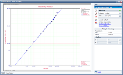
The plot of the solution for this example is shown next.
Special Note About Bias
Estimators (i.e. parameter estimates) have properties such as unbiasedness, minimum variance, sufficiency, consistency, squared error constancy, efficiency and completeness [7][5]. Numerous books and papers deal with these properties and this coverage is beyond the scope of this reference.
However, we would like to briefly address one of these properties, unbiasedness. An estimator is said to be unbiased if the estimator [math]\displaystyle{ \widehat{\theta }=d({{X}_{1,}}{{X}_{2,}}...,{{X}_{n)}} }[/math] satisfies the condition [math]\displaystyle{ E\left[ \widehat{\theta } \right] }[/math] [math]\displaystyle{ =\theta }[/math] for all [math]\displaystyle{ \theta \in \Omega . }[/math] Note that [math]\displaystyle{ E\left[ X \right] }[/math] denotes the expected value of X and is defined (for continuous distributions) by:
- [math]\displaystyle{ \begin{align} E\left[ X \right]= \int_{\varpi }x\cdot f(x)dx \\ X\in & \varpi . \end{align} }[/math]
It can be shown [7][5] that the MLE estimator for the mean of the normal (and lognormal) distribution does satisfy the unbiasedness criteria, or [math]\displaystyle{ E\left[ \widehat{\mu } \right] }[/math] [math]\displaystyle{ =\mu . }[/math] The same is not true for the estimate of the variance [math]\displaystyle{ \hat{\sigma }_{T}^{2} }[/math] . The maximum likelihood estimate for the variance for the normal distribution is given by:
- [math]\displaystyle{ \hat{\sigma }_{T}^{2}=\frac{1}{N}\underset{i=1}{\overset{N}{\mathop \sum }}\,{{({{T}_{i}}-\bar{T})}^{2}} }[/math]
with a standard deviation of:
- [math]\displaystyle{ {{\hat{\sigma }}_{T}}=\sqrt{\frac{1}{N}\underset{i=1}{\overset{N}{\mathop \sum }}\,{{({{T}_{i}}-\bar{T})}^{2}}} }[/math]
These estimates, however, have been shown to be biased. It can be shown [7][5] that the unbiased estimate of the variance and standard deviation for complete data is given by:
- [math]\displaystyle{ \begin{align} \hat{\sigma }_{T}^{2}= & \left[ \frac{N}{N-1} \right]\cdot \left[ \frac{1}{N}\underset{i=1}{\overset{N}{\mathop \sum }}\,{{({{T}_{i}}-\bar{T})}^{2}} \right]=\frac{1}{N-1}\underset{i=1}{\overset{N}{\mathop \sum }}\,{{({{T}_{i}}-\bar{T})}^{2}} \\ {{{\hat{\sigma }}}_{T}}= & \sqrt{\left[ \frac{N}{N-1} \right]\cdot \left[ \frac{1}{N}\underset{i=1}{\overset{N}{\mathop \sum }}\,{{({{T}_{i}}-\bar{T})}^{2}} \right]} \\ = & \sqrt{\frac{1}{N-1}\underset{i=1}{\overset{N}{\mathop \sum }}\,{{({{T}_{i}}-\bar{T})}^{2}}} \end{align} }[/math]
Note that for larger values of [math]\displaystyle{ N }[/math] , [math]\displaystyle{ \sqrt{\left[ N/(N-1) \right]} }[/math] tends to 1.
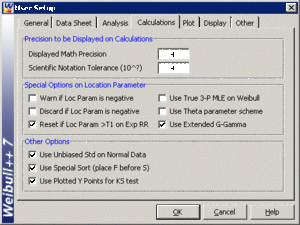
Weibull++ by default returns the standard deviation as defined by Eqn. (NormSt2). The Use Unbiased Std on Normal Data option in the User Setup under the Calculations tab allows biasing to be considered when estimating the parameters.
When this option is selected, Weibull++ returns the standard deviation as defined by Eqn. (NormSt2). This is only true for complete data sets. For all other data types, Weibull++ by default returns the standard deviation as defined by Eqn. (normbias2) regardless of the selection status of this option. The next figure shows this setting in Weibull++.
[math]\displaystyle{ }[/math]


